M8 · Migration from siteBayes2 • multisiteDGP

Abstract

For users of the internal siteBayes2 package who need to migrate scripts to multisiteDGP. The new package keeps the data-generating process and drops the Stan-based fitting, so the migration is mostly a rename map plus a removal list. You leave with eight worked before/after patterns, a function rename table, an explicit deprecated-functions table that points to downstream Bayesian packages, and the boundary check confirming siteBayes2 exports are absent from the multisiteDGP namespace.

1. Scope of the migration

multisiteDGP carries forward the data-generating process from siteBayes2 and leaves Bayesian fitting to downstream packages. Two practical consequences for an existing script:

Renamed surface. sim_multisite_data(), gen_priorG(), sim_sitesize_withinvar(), sim_observed_effects(), get_shrinkage_factor() and friends become sim_multisite(), gen_effects(), gen_site_sizes(), align_rank_corr() plus gen_observations(), and mean_shrinkage() — same idea, cleaner separation across the four generative layers (Lee et al., 2025).
Removed surface. fit_rubin_normal(), lm_stan(), data_prep_rubin_normal() and the inst/stan/ model objects do not move. multisiteDGP installs without a C++ compiler. Fit with metafor, baggr, or rstan directly via the adapters in M6: Adapters and downstream packages.

Sections 2 and 3 give the rename and removal tables. Sections 4 through 11 walk through eight before/after patterns (MV1–MV8) — each runs as printed. Sections 12 and 13 cover the boundary check and where to read next.

2. Function rename map

The canonical translation from siteBayes2 to multisiteDGP. Every target name in the right column appears in NAMESPACE; verify with grep '^export' multisiteDGP-R-package/NAMESPACE.

siteBayes2	multisiteDGP	Notes
`sim_multisite_data()`	`sim_multisite()`	Front door; refactored into the four-layer pipeline
`gen_priorG()`	`gen_effects()`	Layer 1; selects from eight built-in $G$ shapes
`gen_priorG2()`	`gen_effects()` with `formula`, `beta`, `data`	Same function; covariate-aware path is an argument set, not a separate function
`sim_sitesize_withinvar()`	`gen_site_sizes()`	Layer 2; engine choice replaces the implicit JEBS algorithm
`sim_observed_effects()`	`align_rank_corr()` + `gen_observations()`	Layer 3 (dependence) and Layer 4 (observation) are now explicit
`get_shrinkage_factor()`	`mean_shrinkage()`	Vectorized over `nj_mean`; returns the mean-shrinkage scalar diagnostic
`precision_dependence = TRUE`	`sim_multisite()` with `dependence = "rank"` and `rank_corr`	Three named injection methods replace the boolean flag
`precision_dependence = FALSE`	`sim_multisite()` with `dependence = "none"` (default)	Same intent: precision and effect are sampled independently

3. Deprecated functions — no equivalent in multisiteDGP

The Stan-based fitting surface is intentionally absent. There is no shim and no compatibility layer in multisiteDGP itself; downstream packages are the destination.

siteBayes2	Where to go now	Why removed
`fit_rubin_normal()`	`metafor::rma()` after `as_metafor()`; `baggr::baggr()` after `as_baggr()`	Frequentist and Bayesian random-effects fitting are first-class in `metafor`/`baggr`
`lm_stan()`	`rstanarm::stan_lm()`, `brms::brm()`	General-purpose Bayesian linear regression belongs in a general-purpose package
`data_prep_rubin_normal()`	`as_metafor()`, `as_baggr()`	The adapter renames effect, SE, and site columns to the target convention
`prior_rubin_normal()`	`baggr::baggr()` argument `prior_hypermean`, `prior_hypersd`	Prior elicitation is the fitting package’s responsibility
`inst/stan/`, `src/`	`rstan::stan_model()`, `cmdstanr::cmdstan_model()` (user-managed)	multisiteDGP installs without a C++ compiler; no compiled artifacts ship
`pp_check_rubin_normal()`	`bayesplot::pp_check()`, `posterior::summarise_draws()`	Posterior diagnostics belong with the posterior, not the DGP
`loo_rubin_normal()`	`loo::loo()` on the fit object	Model comparison is downstream of fitting

The split makes both packages smaller. multisiteDGP is pure R and ships only the four generative layers plus diagnostics; whichever Bayesian engine fits best for a project lives in that engine’s package, not in a vendor lock-in wrapper (Walters, 2024).

4. MV1 — front door

The monolithic sim_multisite_data() call with many flat arguments becomes either a preset piped into sim_multisite() or a direct call with the same flat arguments.

Before (siteBayes2):

library(siteBayes2)

df_old <- sim_multisite_data(
  true_dist            = "Mixture",
  J                    = 50,
  sigma_tau            = 0.20,
  delta                = 5,
  eps                  = 0.3,
  ups                  = 2,
  nj_mean              = 40,
  cv                   = 0.50,
  nj_min               = 5,
  precision_dependence = FALSE,
  set_seed             = TRUE
)

After (multisiteDGP — preset path):

dat <- preset_jebs_paper() |>
  sim_multisite(seed = 123L)
print(dat, n = 3)
#> # A multisitedgp_data: 50 sites, paradigm = "site_size"
#> # Realized vs intended:
#> #   I: realized=0.243 (no target)
#> #   R: realized=17.000 (no target)
#> #   sigma_tau: target=0.200, realized=0.199, PASS
#> #   rho_S: target=0.000, realized=0.130, PASS
#> #   rho_S_marg: realized=0.130 (no target)
#> #   Feasibility: WARN (n_eff=12.853)
#> # A tibble: 50 × 7
#>   site_index    z_j  tau_j tau_j_hat  se_j se2_j   n_j
#>        <int>  <dbl>  <dbl>     <dbl> <dbl> <dbl> <int>
#> 1          1 -1.19  -0.238   -0.0622 0.392 0.154    26
#> 2          2  1.10   0.219   -0.0135 0.603 0.364    11
#> 3          3 -0.504 -0.101   -0.886  0.5   0.25     16
#> # ℹ 47 more rows
#> # Use summary(df) for the full diagnostic report.

The print method displays realized vs. intended diagnostics (informativeness $I$ , heterogeneity ratio $R$ , residual heterogeneity $\sigma_\tau$ , rank correlation $\rho_S$ ). preset_jebs_paper() is the JEBS replication preset; the sim_multisite() front door applies it through the four layers.

5. MV2 — flat JEBS-style arguments

When the script needs the arguments visible (e.g. for a sweep), pass them directly to sim_multisite(). The mixture parameters now live inside theta_G; everything else is a named argument with the original meaning.

flat_dat <- sim_multisite(
  J         = 50L,
  true_dist = "Mixture",
  theta_G   = list(delta = 5, eps = 0.3, ups = 2),
  sigma_tau = 0.20,
  nj_mean   = 40,
  cv        = 0.50,
  nj_min    = 5L,
  engine    = "A1_legacy",
  dependence = "none",
  seed      = 123L
)
head(tibble::as_tibble(flat_dat)[, c("site_index", "z_j", "tau_j", "tau_j_hat", "se2_j")], 3)
#> # A tibble: 3 × 5
#>   site_index    z_j  tau_j tau_j_hat se2_j
#>        <int>  <dbl>  <dbl>     <dbl> <dbl>
#> 1          1 -1.19  -0.238   -0.0622 0.154
#> 2          2  1.10   0.219   -0.0135 0.364
#> 3          3 -0.504 -0.101   -0.886  0.25

engine = "A1_legacy" reproduces the original siteBayes2 site-size algorithm (truncated-and-rounded gamma); the default engine = "A2_modern" uses moment-matched truncated gamma — both hit the same (nj_mean, cv) target, but the legacy engine matches JEBS Table 3 row-for-row (Lee et al., 2025). See M2: G-distribution catalog for the $G$ -shape parameter convention theta_G enforces.

6. MV3 — covariate-aware and custom $G$

gen_priorG() and gen_priorG2() collapse to a single gen_effects(). The covariate-aware path is an argument set (formula, beta, data), not a separate function.

x <- data.frame(X1 = as.numeric(scale(seq_len(30L))))
effects <- gen_effects(
  J         = 30L,
  true_dist = "Gaussian",
  sigma_tau = 0.15,
  formula   = ~ X1,
  beta      = 0.30,
  data      = x
)
head(effects, 3)
#> # A tibble: 3 × 4
#>   site_index    z_j  tau_j    X1
#>        <int>  <dbl>  <dbl> <dbl>
#> 1          1 -0.626 -0.588 -1.65
#> 2          2  0.184 -0.433 -1.53
#> 3          3 -0.836 -0.551 -1.42

For a non-built-in $G$ , switch to true_dist = "User" and pass g_fn. The callback returns standardized residuals by default; multisiteDGP audits and rescales them.

my_g <- function(J, ...) {
  z <- stats::rt(J, df = 5)
  (z - mean(z)) / stats::sd(z)
}
custom_dat <- sim_multisite(
  multisitedgp_design(
    J         = 40L,
    true_dist = "User",
    g_fn      = my_g,
    g_returns = "standardized"
  ),
  seed = 44L
)
informativeness(custom_dat)
#> [1] 0.2984526

The full custom- $G$ contract — including the g_returns = "raw" escape hatch — is in M5: Custom G distributions. The eight built-in shapes are catalogued in M2: G-distribution catalog, which includes the gen_priorG rename map under each shape.

7. MV4 — split dependence and observation

sim_observed_effects() used to combine dependence alignment and observation sampling. multisiteDGP keeps those layers separate so each can be inspected, customized, or audited.

effects   <- gen_effects_gaussian(J = 20L, sigma_tau = 0.20)
margins   <- gen_site_sizes(effects, J = 20L, nj_mean = 50, cv = 0.30)
dependent <- align_rank_corr(margins, rank_corr = 0.30, max_iter = 2000L)
observed  <- gen_observations(dependent)

stats::cor(observed$z_j, observed$se2_j, method = "spearman")
#> [1] 0.3002258
head(observed, 3)
#> # A tibble: 3 × 7
#>   site_index    z_j   tau_j   n_j  se2_j  se_j tau_j_hat
#>        <int>  <dbl>   <dbl> <int>  <dbl> <dbl>     <dbl>
#> 1          1  1.36   0.272     42 0.0952 0.309     0.418
#> 2          2 -0.103 -0.0206    54 0.0741 0.272    -0.214
#> 3          3  0.388  0.0775    58 0.0690 0.263     0.238

Most users should still call sim_multisite(); the layered calls are useful when migrating custom internals or when swapping a single layer (e.g. a copula dependence injection in place of rank-corr alignment).

8. MV5 — Stan fitting moves downstream

multisiteDGP does not ship Stan models, Rcpp code, or Bayesian fitting wrappers. The package installs without a C++ compiler.

Before (siteBayes2):

library(siteBayes2)
fit_old <- fit_rubin_normal(
  df          = sites,
  tau_hat_col = "tau_j_hat",
  se2_col     = "se2_j",
  iter        = 2000,
  chains      = 4
)

After (multisiteDGP — adapter to metafor):

fit_dat <- sim_multisite(J = 30L, seed = 1L)

if (requireNamespace("metafor", quietly = TRUE)) {
  meta_dat <- as_metafor(fit_dat)
  fit_meta <- metafor::rma(yi = meta_dat$yi, vi = meta_dat$vi, method = "REML")
  print(fit_meta)
} else {
  message("Install metafor for the random-effects fit: install.packages('metafor')")
}
#> 
#> Random-Effects Model (k = 30; tau^2 estimator: REML)
#> 
#> tau^2 (estimated amount of total heterogeneity): 0.0419 (SE = 0.0334)
#> tau (square root of estimated tau^2 value):      0.2047
#> I^2 (total heterogeneity / total variability):   32.89%
#> H^2 (total variability / sampling variability):  1.49
#> 
#> Test for Heterogeneity:
#> Q(df = 29) = 43.3550, p-val = 0.0422
#> 
#> Model Results:
#> 
#> estimate      se    zval    pval    ci.lb   ci.ub    
#>   0.0342  0.0662  0.5162  0.6057  -0.0956  0.1639    
#> 
#> ---
#> Signif. codes:  0 '***' 0.001 '**' 0.01 '*' 0.05 '.' 0.1 ' ' 1

The adapter renames the canonical columns to metafor’s (yi, vi, sei) convention without touching the numerical values. The full contract is in M6: Adapters and downstream packages.

9. MV6 — `baggr` path

Bayesian random-effects fitting through baggr follows the same pattern: adapt, then fit. include_truth = TRUE keeps tau_j as tau_true so post-fit recovery checks are one column away.

if (requireNamespace("baggr", quietly = TRUE)) {
  bg <- as_baggr(fit_dat, include_truth = TRUE)
  head(bg, 3)
} else {
  message("Install baggr for the Bayesian random-effects fit: install.packages('baggr')")
}
#> # A tibble: 3 × 3
#>      tau    se tau_true
#>    <dbl> <dbl>    <dbl>
#> 1 0.923  0.436  -0.125 
#> 2 0.0266 0.258   0.0367
#> 3 0.0320 0.289  -0.167

as_baggr() renames to (tau, se, tau_true). The fit call itself is baggr::baggr(bg) — multisiteDGP does not wrap it.

10. MV7 — shrinkage helper

get_shrinkage_factor() is replaced by mean_shrinkage(), now vectorized over nj_mean.

mean_shrinkage(
  nj_mean   = c(20, 50, 100),
  sigma_tau = 0.15,
  varY      = 1,
  p         = 0.5,
  R2        = 0.20
)
#> [1] 0.1232877 0.2601156 0.4128440

The three values are the mean shrinkage factors at $\bar n_j = 20, 50, 100$ . Larger sites see stronger shrinkage toward the global mean. The diagnostic also has a multisitedgp_data method that reads varY and p from the design’s provenance.

11. MV8 — no legacy exports in multisiteDGP

multisiteDGP intentionally does not export siteBayes2 names. That keeps the new package small, pure-R, and DGP-only. If a script needs backwards compatibility, the place for that is a thin siteBayes2-compatibility patch package that imports multisiteDGP and issues deprecation warnings — not multisiteDGP itself.

legacy_names <- c(
  "sim_multisite_data",
  "gen_priorG",
  "gen_priorG2",
  "sim_sitesize_withinvar",
  "sim_observed_effects",
  "get_shrinkage_factor"
)
legacy_names %in% getNamespaceExports("multisiteDGP")
#> [1] FALSE FALSE FALSE FALSE FALSE FALSE

All six return FALSE, confirming the boundary.

12. Realized-design check on a migrated script

A migrated script should be checked the same way an originally-written multisiteDGP script is — by reading the realized-vs.-intended diagnostic block and the funnel plot. The two together confirm that the new pipeline reproduces the design intent of the old call.

migrated <- preset_jebs_paper() |> sim_multisite(seed = 123L)
summary(migrated)
#> multisiteDGP simulation diagnostics
#> ------------------------------------------------------------
#> A. Realized vs Intended
#>    I (informativeness):         0.243  (target N/A)  N/A   [no target]
#>    R (SE heterogeneity):       17.000  (target N/A)  N/A   [no target]
#>    sigma_tau:                   0.199  (target 0.200)  PASS  [rel=-0.4%]
#>    GM(se^2):                    0.125  (target N/A)  N/A   [no target]
#> 
#> B. Dependence
#>    rank_corr residual:          0.130  (target 0.000)  PASS  [delta=0.130]
#>    rank_corr marginal:          0.130  (target N/A)  N/A   [residual target rows only; no finite target; status not assigned]
#>    pearson_corr residual:       0.034  (target 0.000)  WARN  [delta=0.034]
#>    pearson_corr marginal:       0.034  (target N/A)  N/A   [residual target rows only; no finite target; status not assigned]
#> 
#> C. G shape fit
#>    KS distance D_J:               N/A  (target 0.000)  N/A   [no target]
#>    Bhattacharyya BC:              N/A  (target 1.000)  N/A   [no target]
#>    Q-Q residual:                  N/A  (target 0.000)  N/A   [order-statistic band metadata deferred]
#> 
#> D. Operational feasibility
#>    mean shrinkage S:            0.257  (target N/A)  PASS  [no target]
#>    avg MOE (95%):               0.722  (target N/A)  WARN  [no target]
#>    feasibility_index:          12.853  (target N/A)  WARN  [no target]
#> ------------------------------------------------------------
#> Overall: 3 PASS, 3 WARN, 0 FAIL.
#> Provenance: multisiteDGP 0.1.1 | paradigm=site_size | seed=123 | canonical_hash=7bb08e59be82c6e7 | design_hash=e3b4a0a694b82f67 | hash_algo=xxhash64 | R=4.6.0 | hooks=none

plot_funnel(migrated)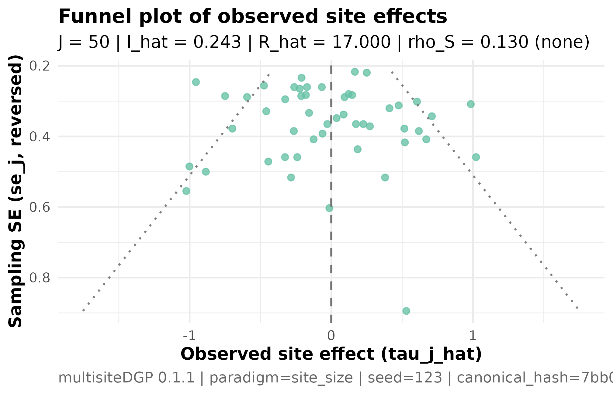

Funnel plot with site SE on the x-axis and observed effect on the y-axis. Points fan out symmetrically as SE grows.

Funnel plot of the migrated JEBS-preset simulation. Each point is a site; horizontal axis is the site SE, vertical axis is the observed estimate tau_j_hat. The funnel widens with SE as expected under the canonical factorization $y_j = \tau_j + e_j,\, e_j \sim \mathcal{N}(0,\sigma_j^2)$ . No high-precision sites cluster at extreme estimates and no low-precision sites cluster near zero, confirming the migrated pipeline preserves the precision-effect independence target $\rho_S = 0$ .

The diagnostic block reports realized $\sigma_\tau = 0.199$ against the target $0.200$ (PASS) and realized $\rho_S = 0.130$ against the target $0.000$ (PASS within tolerance). The funnel plot is the visual companion: symmetric scatter widening with SE confirms the precision-effect independence the JEBS preset targets.

13. Three points where the new API diverges, not just renames

Most patterns above are pure renames. Three are not.

Layer separation (MV4). sim_observed_effects() mixed dependence injection and observation sampling. multisiteDGP separates them into align_rank_corr() / align_copula_corr() / align_hybrid_corr() (Layer 3) and gen_observations() (Layer 4). Three precision-injection methods replace the boolean precision_dependence. The full contract — including which method hits the rank-correlation target most efficiently at given $J$ — is in M4: Precision dependence — three injection methods.
Two front doors, two paradigms (MV2 and MV5). siteBayes2 treated direct-precision designs as a flag. multisiteDGP separates them into two front doors: sim_multisite() for the site-size-driven path (paradigm = "site_size" — sample sizes $n_j$ produce SEs $\sigma_j^2 = \kappa / n_j$ ) and sim_meta() for the direct-precision path (paradigm = "direct" — informativeness $I$ and heterogeneity ratio $R$ produce SEs directly via a geometric grid). The construction-time check redirects mismatches at design time. See M3: Margin and SE models for the formal statement.
g_fn standardization audit (MV3). siteBayes2’s custom $G$ hook accepted any callback. multisiteDGP audits the callback’s output against g_returns = "standardized" (default) or "raw" and rescales to the requested sigma_tau; the audit can be turned off for development work via audit_g = FALSE. See M5: Custom G distributions.

14. Where to next

For an end-to-end migrated workflow:

A1: Getting started — the basic four-step pipeline, the same pipeline a migrated script ends up running.
A2: Choosing a preset — the eight presets cover the JEBS replication, two meta-analytic profiles, and small-area estimation; most migrated scripts can replace a flat argument list with a preset call.

For the methodological mapping behind the renames:

M2: G-distribution catalog — the eight built-in $G$ shapes and the gen_priorG → gen_effects parameter map per shape.
M3: Margin and SE models — the site-size-driven and direct-precision paths, sim_multisite() vs. sim_meta(), and why the two are separated rather than flagged.
M4: Precision dependence — three injection methods — the rank, copula, and hybrid alternatives that replace precision_dependence = TRUE/FALSE.

References

The two-stage data-generating process and the canonical factorization $y_j = \tau_j + e_j$ that the renamed function set implements is from Lee et al. (2025). The empirical-Bayes shrinkage target the migrated adapter pipeline produces is the analysis goal in Walters (2024).

Acknowledgments

This research was supported by the Institute of Education Sciences, U.S. Department of Education, through Grant R305D240078 to the University of Alabama. The opinions expressed are those of the authors and do not represent views of the Institute or the U.S. Department of Education.

Session info

#> R version 4.6.0 (2026-04-24)
#> Platform: x86_64-pc-linux-gnu
#> Running under: Ubuntu 24.04.4 LTS
#> 
#> Matrix products: default
#> BLAS:   /usr/lib/x86_64-linux-gnu/openblas-pthread/libblas.so.3 
#> LAPACK: /usr/lib/x86_64-linux-gnu/openblas-pthread/libopenblasp-r0.3.26.so;  LAPACK version 3.12.0
#> 
#> locale:
#>  [1] LC_CTYPE=C.UTF-8       LC_NUMERIC=C           LC_TIME=C.UTF-8       
#>  [4] LC_COLLATE=C.UTF-8     LC_MONETARY=C.UTF-8    LC_MESSAGES=C.UTF-8   
#>  [7] LC_PAPER=C.UTF-8       LC_NAME=C              LC_ADDRESS=C          
#> [10] LC_TELEPHONE=C         LC_MEASUREMENT=C.UTF-8 LC_IDENTIFICATION=C   
#> 
#> time zone: UTC
#> tzcode source: system (glibc)
#> 
#> attached base packages:
#> [1] stats     graphics  grDevices utils     datasets  methods   base     
#> 
#> other attached packages:
#> [1] ggplot2_4.0.3      multisiteDGP_0.1.1
#> 
#> loaded via a namespace (and not attached):
#>  [1] gtable_0.3.6          xfun_0.57             bslib_0.10.0         
#>  [4] QuickJSR_1.9.2        ggrepel_0.9.8         inline_0.3.21        
#>  [7] lattice_0.22-9        mathjaxr_2.0-0        numDeriv_2016.8-1.1  
#> [10] vctrs_0.7.3           tools_4.6.0           generics_0.1.4       
#> [13] yulab.utils_0.2.4     parallel_4.6.0        stats4_4.6.0         
#> [16] tibble_3.3.1          pkgconfig_2.0.3       Matrix_1.7-5         
#> [19] checkmate_2.3.4       ggplotify_0.1.3       RColorBrewer_1.1-3   
#> [22] S7_0.2.2              desc_1.4.3            RcppParallel_5.1.11-2
#> [25] lifecycle_1.0.5       compiler_4.6.0        farver_2.1.2         
#> [28] textshaping_1.0.5     codetools_0.2-20      forestplot_3.2.0     
#> [31] htmltools_0.5.9       sass_0.4.10           bayesplot_1.15.0     
#> [34] yaml_2.3.12           pillar_1.11.1         pkgdown_2.2.0        
#> [37] crayon_1.5.3          jquerylib_0.1.4       cachem_1.1.0         
#> [40] StanHeaders_2.32.10   metadat_1.6-0         abind_1.4-8          
#> [43] nlme_3.1-169          rstan_2.32.7          tidyselect_1.2.1     
#> [46] digest_0.6.39         dplyr_1.2.1           labeling_0.4.3       
#> [49] fastmap_1.2.0         grid_4.6.0            cli_3.6.6            
#> [52] metafor_5.0-1         magrittr_2.0.5        loo_2.9.0            
#> [55] pkgbuild_1.4.8        withr_3.0.2           scales_1.4.0         
#> [58] backports_1.5.1       rappdirs_0.3.4        rmarkdown_2.31       
#> [61] matrixStats_1.5.0     gridExtra_2.3         ragg_1.5.2           
#> [64] evaluate_1.0.5        knitr_1.51            baggr_0.8            
#> [67] nleqslv_3.3.7         gridGraphics_0.5-1    rstantools_2.6.0     
#> [70] rlang_1.2.0           Rcpp_1.1.1-1.1        glue_1.8.1           
#> [73] jsonlite_2.0.0        R6_2.6.1              systemfonts_1.3.2    
#> [76] fs_2.1.0

Lee, J., Che, J., Rabe-Hesketh, S., Feller, A., & Miratrix, L. (2025). Improving the estimation of site-specific effects and their distribution in multisite trials. Journal of Educational and Behavioral Statistics, 50(5), 731–764. https://doi.org/10.3102/10769986241254286

Walters, C. (2024). Empirical bayes methods in labor economics. In Handbook of labor economics (Vol. 5, pp. 183–260). Elsevier. https://doi.org/10.1016/bs.heslab.2024.11.001

M8 · Migration from siteBayes2

JoonHo Lee

2026-05-10

1. Scope of the migration

2. Function rename map

3. Deprecated functions — no equivalent in multisiteDGP

4. MV1 — front door

5. MV2 — flat JEBS-style arguments

6. MV3 — covariate-aware and custom $G$

7. MV4 — split dependence and observation

8. MV5 — Stan fitting moves downstream

9. MV6 — `baggr` path

10. MV7 — shrinkage helper

11. MV8 — no legacy exports in multisiteDGP

12. Realized-design check on a migrated script

13. Three points where the new API diverges, not just renames

14. Where to next

References

Acknowledgments

Session info

M8 · Migration from siteBayes2

JoonHo Lee

2026-05-10

1. Scope of the migration

2. Function rename map

3. Deprecated functions — no equivalent in multisiteDGP

4. MV1 — front door

5. MV2 — flat JEBS-style arguments

6. MV3 — covariate-aware and custom GG

7. MV4 — split dependence and observation

8. MV5 — Stan fitting moves downstream

9. MV6 — baggr path

10. MV7 — shrinkage helper

11. MV8 — no legacy exports in multisiteDGP

12. Realized-design check on a migrated script

13. Three points where the new API diverges, not just renames

14. Where to next

References

Acknowledgments

Session info

6. MV3 — covariate-aware and custom $G$

9. MV6 — `baggr` path