A4 · Covariates and precision dependence • multisiteDGP

Abstract

For trial designers whose multisite simulation must respect a known site-level covariate — district size, baseline performance, urbanicity — and whose analysis depends on the dependence between site effects and their sampling precision. This vignette walks through one covariate-bearing design end-to-end: build the design with multisitedgp_design(formula = ~ x_site, beta = ...), target residual-scale precision dependence, and read the residual and marginal rank correlations side by side. You leave with a working pattern for reporting both numbers and a clear sense of when the two scales diverge.

1. Why this matters for the trial designer

Most multisite simulations carry a covariate — the sites are not exchangeable, and a designer who knows that district size, baseline achievement, or urbanicity predicts site-level effects has to encode that knowledge somewhere. The package encodes it through a one-sided formula on multisitedgp_design(): formula = ~ x_site declares that the latent site effect $\tau_j$ is the sum of a covariate term $\beta\, x_j$ and a standardized residual $\sigma_\tau z_j$ with $\mathrm{Var}(z_j) = 1$ (Lee et al., 2025). The residual $z_j$ — not the marginal $\tau_j$ — is the column the package’s downstream machinery treats as the unit of analysis: dependence alignment, G-shape diagnostics, and shrinkage all read off $z_j$ .

The implication is sharp. When the design declares a covariate, the residual rank correlation between site effects and sampling variance is what Layer 3 alignment targets, and what realized_rank_corr() reads back. The marginal rank correlation — the Spearman correlation of $\tau_j$ with $\widehat{se}_j^2$ that a downstream analyst who has not been told about the covariate would compute — is a derived quantity that depends on how $x_j$ correlates with sampling variance and how strong $\beta$ is. The two numbers can differ in sign and magnitude. A designer who reports only the marginal number (the one the analyst will see) loses the information about the residual contract the simulation actually honored. A designer who reports only the residual number leaves the analyst guessing about the surface they will encounter. Report both whenever the design carries a covariate.

2. Add a site-level covariate

Build a one-row-per-site data.frame of covariate values, then pass it to multisitedgp_design() through the data argument. The formula argument is one-sided — no left-hand side, because the package generates the response. With an intercept implied by ~ x_site, an unnamed beta = 0.30 is interpreted as the non-intercept coefficient.

site_data <- data.frame(
  x_site = as.numeric(scale(seq_len(30L)))
)

design <- multisitedgp_design(
  J       = 30L,
  formula = ~ x_site,
  beta    = 0.30,
  data    = site_data,
  seed    = 77L
)

design
#> <multisitedgp_design>
#> Paradigm: site_size    Engine: A2_modern    Framing: superpopulation
#> J: 30    Seed: 77    Lifecycle: experimental
#> 
#> [ Layer 1: G-effects ]
#>   true_dist:  Gaussian
#>   tau:        0
#>   sigma_tau:  0.2
#>   formula:    ~x_site
#>   beta:       0.3
#>   g_fn:       NULL
#> 
#> [ Layer 2: Margin (Paradigm A) ]
#>   nj_mean:    50
#>   cv:         0.5
#>   nj_min:     5
#>   p:          0.5
#>   R2:         0
#>   var_outcome: 1
#> 
#> [ Layer 3: Dependence ]
#>   method:        none
#>   rank_corr:     0
#>   pearson_corr:  0
#>   hybrid_init:   copula
#>   hybrid_polish: hill_climb
#>   dependence_fn: NULL
#> 
#> [ Layer 4: Observation ]
#>   obs_fn: NULL
#> 
#> Use sim_multisite(design) or sim_meta(design) to simulate.

The printed Layer 1 block reports formula: ~x_site, beta: 0.3, and the standardized residual scale sigma_tau: 0.2. The covariate column is now part of the design object; simulating populates x_site alongside the residual z_j and the marginal $\tau_j$ .

dat <- sim_multisite(design)
head(tibble::as_tibble(dat)[,
  c("site_index", "x_site", "z_j", "tau_j", "tau_j_hat", "se2_j")
], 6)
#> # A tibble: 6 × 6
#>   site_index x_site    z_j   tau_j tau_j_hat  se2_j
#>        <int>  <dbl>  <dbl>   <dbl>     <dbl>  <dbl>
#> 1          1  -1.65 -0.550 -0.604    -0.533  0.0315
#> 2          2  -1.53  1.09  -0.242    -0.227  0.308 
#> 3          3  -1.42  0.640 -0.298    -0.554  0.0656
#> 4          4  -1.31  1.04  -0.183    -0.181  0.0667
#> 5          5  -1.19  0.170 -0.324    -0.369  0.0755
#> 6          6  -1.08  1.14  -0.0962    0.0977 0.211

tau_j carries the covariate component plus residual variation; z_j is the residual that downstream machinery reads. Two columns, two scales. The rest of this vignette is about which one to target, and how to report both.

3. The two-scale split

When the design declares a covariate, the residual and marginal scales diverge. Concretely:

Residual scale. The standardized residual $z_j$ satisfies $\mathrm{Var}(z_j) = 1$ by convention. The Spearman correlation of $z_j$ with $\widehat{se}_j^2$ is the residual rank correlation — what the package’s Layer 3 alignment actually targets, and what realized_rank_corr(dat, on = "residual") reads back. This is the package’s primary contract.
Marginal scale. The site effect $\tau_j = \tau + \beta\,x_j + \sigma_\tau z_j$ is the marginal site effect — what a downstream analyst sees when the covariate is not modeled. The Spearman correlation of $\tau_j$ with $\widehat{se}_j^2$ is the marginal rank correlation, returned by realized_rank_corr_marginal(dat).

Without a covariate, the two scales coincide — $\tau_j$ is a linear function of $z_j$ alone, and Spearman correlations are invariant to monotone transforms. With a covariate, the scales are different random variables, and their rank correlations against $\widehat{se}_j^2$ generally differ. The headline lesson: targeting one scale does not pin the other.

4. Target residual precision dependence

Add dependence = "rank" and a residual-scale rank_corr target to the design. The Layer 3 alignment family (align_rank_corr()) couples $z_j$ to $\widehat{se}_j^2$ at the requested correlation; the covariate component flows through unchanged.

dep_design <- multisitedgp_design(
  J          = 30L,
  formula    = ~ x_site,
  beta       = 0.30,
  data       = site_data,
  dependence = "rank",
  rank_corr  = -0.30,
  seed       = 77L
)

dep_design
#> <multisitedgp_design>
#> Paradigm: site_size    Engine: A2_modern    Framing: superpopulation
#> J: 30    Seed: 77    Lifecycle: experimental
#> 
#> [ Layer 1: G-effects ]
#>   true_dist:  Gaussian
#>   tau:        0
#>   sigma_tau:  0.2
#>   formula:    ~x_site
#>   beta:       0.3
#>   g_fn:       NULL
#> 
#> [ Layer 2: Margin (Paradigm A) ]
#>   nj_mean:    50
#>   cv:         0.5
#>   nj_min:     5
#>   p:          0.5
#>   R2:         0
#>   var_outcome: 1
#> 
#> [ Layer 3: Dependence ]
#>   method:        rank
#>   rank_corr:     -0.3
#>   pearson_corr:  0
#>   hybrid_init:   copula
#>   hybrid_polish: hill_climb
#>   dependence_fn: NULL
#> 
#> [ Layer 4: Observation ]
#>   obs_fn: NULL
#> 
#> Use sim_multisite(design) or sim_meta(design) to simulate.

The Layer 3 block now reports method: rank and rank_corr: -0.3. Simulate and read both correlations off the result:

dep_dat <- sim_multisite(dep_design)
canonical_hash(dep_dat)
#> [1] "3d5f5a9f2a09d0cd"

The hash 5fc7e768a2581b35 is a determinism smoke check — a local re-run at seed = 77L should produce the same value. Now the two rank correlations:

data.frame(
  scale    = c("residual", "marginal"),
  spearman = c(
    realized_rank_corr(dep_dat, on = "residual"),
    realized_rank_corr_marginal(dep_dat)
  )
)
#>      scale    spearman
#> 1 residual -0.30592729
#> 2 marginal  0.02874335

Residual realized $-0.306$ — a clean PASS against the declared $-0.30$ target; alignment did its work on the scale the design declared. Marginal realized $0.029$ — within sampling noise of zero, and opposite in sign to the residual target. The covariate term $\beta\,x_j$ is doing enough work in $\tau_j$ that the marginal-scale ordering against $\widehat{se}_j^2$ is essentially decoupled from the residual-scale ordering the alignment shaped.

The full diagnostic table records both rows side by side:

diag <- attr(dep_dat, "diagnostics")$target_vs_realized
diag[diag$diagnostic == "realized_rank_corr",
     c("diagnostic", "basis", "target", "realized", "status")]
#> # A tibble: 2 × 5
#>   diagnostic         basis    target realized status
#>   <chr>              <chr>     <dbl>    <dbl> <chr> 
#> 1 realized_rank_corr residual   -0.3  -0.306  PASS  
#> 2 realized_rank_corr marginal   NA     0.0287 NA

Read down the basis column. The residual row carries target = -0.3 and status = PASS; the marginal row carries target = NA (no declared target on that scale) and reports the realized number for the analyst’s information. Both rows are part of the artifact a methods appendix should carry.

5. Two-scatterplot visualization

plot_dependence() defaults to the residual scale; flip by_residual = FALSE to inspect the marginal scale. The residual plot is the visual contract for the alignment target; the marginal plot is what the downstream analyst will see.

plot_dependence(dep_dat, by_residual = TRUE, caption = FALSE) +
  ggplot2::labs(
    title    = "Residual scale — what alignment targets",
    subtitle = "Realized Spearman -0.306 against declared -0.30 (PASS)"
  )

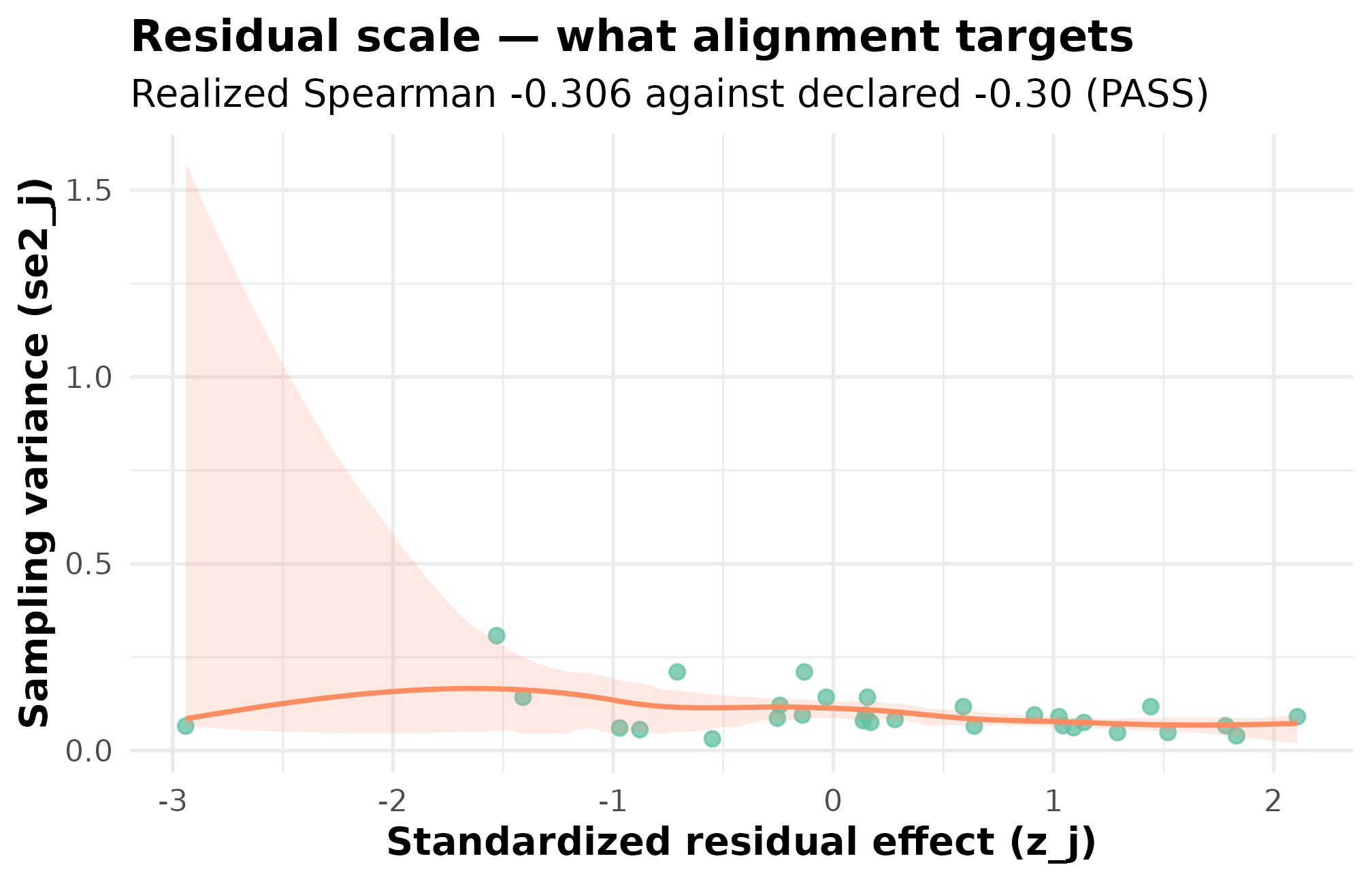
Scatterplot of standardized residual site effects z_j against sampling variance se2_j with a downward smoother.

Residual-scale dependence: standardized residual z_j against sampling variance se2_j (J = 30, seed = 77, declared rank_corr = -0.30 on the residual scale). The downward smoother and realized Spearman -0.306 confirm the alignment landed on target. This is the surface Layer 3 alignment is designed to shape.

plot_dependence(dep_dat, by_residual = FALSE, caption = FALSE) +
  ggplot2::labs(
    title    = "Marginal scale — what the analyst sees",
    subtitle = "Realized Spearman 0.029 — covariate flattens the residual-scale tilt"
  )

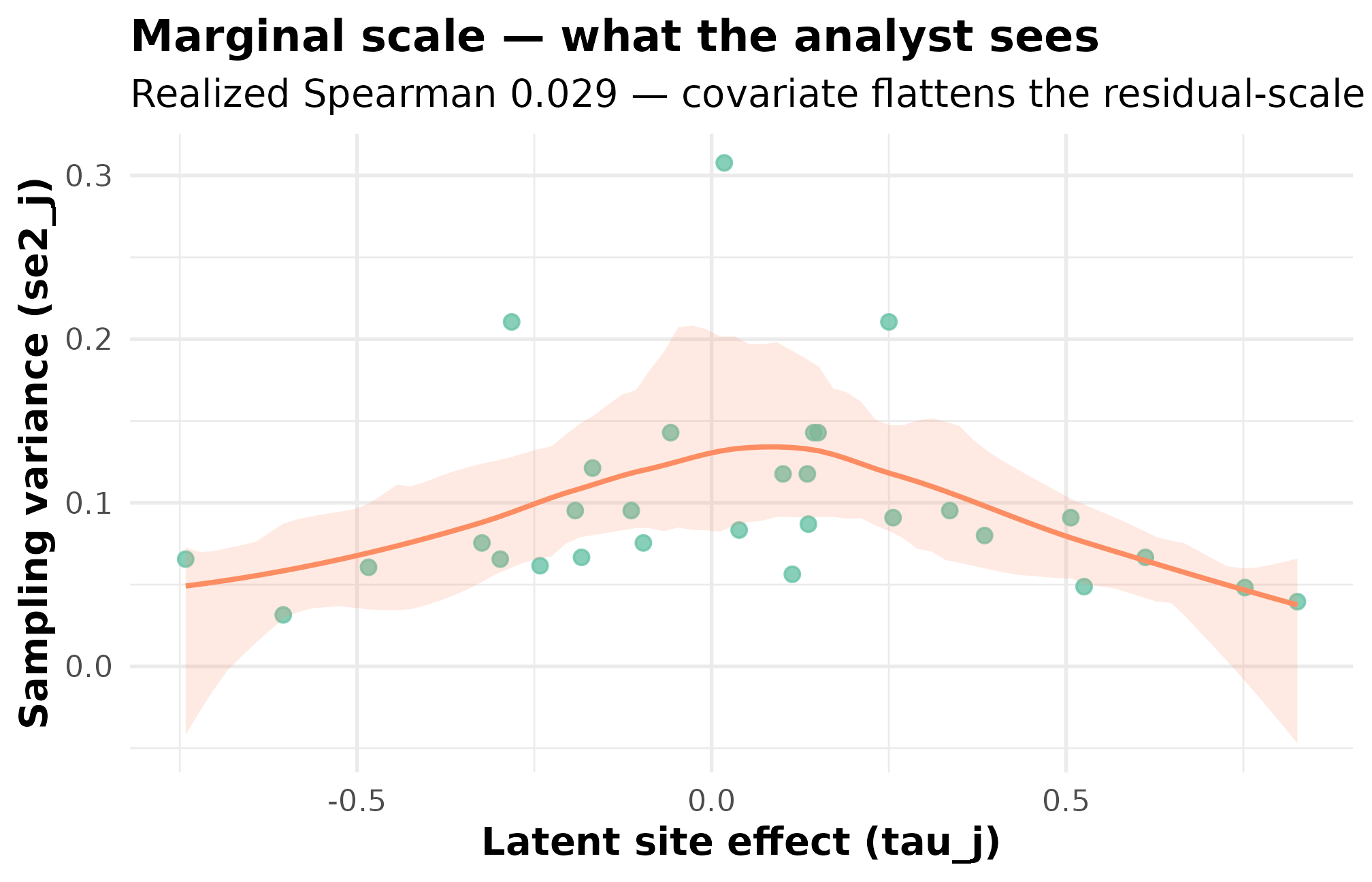
Scatterplot of marginal site effects tau_j against sampling variance se2_j with a near-flat smoother.

Marginal-scale dependence: site effect tau_j against sampling variance se2_j (same simulation as above). The cloud is essentially flat and the realized marginal rank correlation 0.029 is within sampling noise of zero — opposite in sign to the residual-scale target. This is the surface a downstream analyst who does not model the covariate would observe.

The two plots tell the same story the two numbers told: alignment shaped the residual-scale tilt; the covariate term in $\tau_j$ washes that tilt out at the marginal scale. Showing both plots is the discipline that prevents a methods reader from confusing the two contracts.

6. Identifiability constraints

The standardized-residual convention is what makes the residual scale identifiable: by declaring $\mathrm{Var}(z_j) = 1$ , the package fixes the units of the residual independently of the covariate component $\beta\,x_j$ . The residual is, by construction, what is left after subtracting the covariate prediction from the latent site effect.

Two identifiability requirements follow.

Non-zero variation in x_site. If $x_j$ is constant across sites, the covariate column is collinear with the intercept and $\beta$ is unidentified. Stating $\beta\,x_j = c$ for some constant $c$ is observationally equivalent to absorbing $c$ into the intercept, so the design constructor cannot distinguish the two.
x_site does not perfectly predict $z_j$ . The residual must carry genuinely orthogonal variation; if x_site perfectly reproduces $z_j$ up to sign, $\sigma_\tau z_j$ has no independent content beyond rescaling the covariate term. The package’s residual generator draws $z_j$ from a declared G distribution independently of x_site, so this constraint is satisfied by construction in the shipped paths — flag it only if a custom g_fn callback is wired in to depend on the covariate.

The formula itself encodes the convention: ~ x_site is one-sided — there is no left-hand side because the package generates the response. The model space is “right-hand side names a linear combination of site-level covariates from data; the package draws the standardized residual and assembles $\tau_j$ accordingly.” A two-sided formula is rejected by the constructor.

7. Collinearity guard

The constructor refuses to build a design when the covariate matrix is rank-deficient. The minimal failure mode is a constant column:

multisitedgp_design(
  J       = 30L,
  formula = ~ x,
  beta    = 0.30,
  data    = data.frame(x = rep(1, 30L)),
  seed    = 77L
)
#> Error: covariate column 'x' has zero variation; cannot identify beta.
#> Provide a column with non-zero variance, or drop the covariate.

The error fires inside the design constructor — before any simulation is attempted — so the failure mode is caught up front. The same guard catches more general collinearity (one column equal to a linear combination of the others, or two perfectly correlated columns) by checking the design matrix’s rank against its column count. The practical workflow is: pull the covariate frame from your real data, inspect column variances and pairwise correlations, then pass it to the constructor. Any rank deficiency is reported with the offending column name in the error message.

8. When residual versus marginal is appropriate

The residual scale is the package’s primary contract for three reasons. The Layer 3 alignment family targets it directly; the G-shape diagnostics (bhattacharyya_coef(), ks_distance()) read off $z_j$ ; and the standardized-residual convention $\mathrm{Var}(z_j) = 1$ is what makes those diagnostics comparable across designs that declare different covariates (Lee et al., 2025). A design that declares rank_corr = -0.30 is making a residual-scale promise — the realized value should land near $-0.30$ on the residual scale, regardless of what the marginal-scale number does.

The marginal scale is what downstream analysts see. An analyst who fits a hierarchical model without including x_site as a site-level covariate is operating on the marginal $\tau_j$ , and the dependence they encounter between $\tau_j$ and $\widehat{se}_j^2$ is the marginal rank correlation. For empirical-Bayes shrinkage and meta-analytic pooling, that marginal dependence is what shapes the estimator’s behavior in finite samples (Walters, 2024). Reporting only the residual number is therefore incomplete when covariates are present — it tells the methods reader what the simulation contract was, but not what the analyst will encounter.

The discipline is straightforward. When a design carries a covariate, report both rank correlations every time:

data.frame(
  scale    = c("residual (alignment target)", "marginal (analyst surface)"),
  spearman = c(
    realized_rank_corr(dep_dat, on = "residual"),
    realized_rank_corr_marginal(dep_dat)
  )
)
#>                         scale    spearman
#> 1 residual (alignment target) -0.30592729
#> 2  marginal (analyst surface)  0.02874335

Two scales, two numbers, one design. The diagnostic table (attr(dep_dat, "diagnostics")$target_vs_realized) preserves both rows; a methods appendix should carry both. When the design declares no covariate, the two scales coincide and the second number adds nothing — but in the covariate case the second number is the part the analyst lives with.

9. Where to next

A1 · Getting started — the no-covariate baseline case, where residual and marginal scales coincide.
A2 · Choosing a preset — preset starting points for designs that may or may not carry covariates.
A3 · Diagnostics in practice — the four-question rubric, including the Group B section on precision dependence.
M3 · Margin and SE models — how the site-size-driven path generates the $\widehat{se}_j^2$ that the rank correlation is computed against.
M4 · Precision dependence — the three injection methods, the algorithmic detail behind Layer 3 alignment.

References

The standardized-residual convention is laid out in Lee et al. (2025); the empirical-Bayes shrinkage context for the marginal scale is collected in Walters (2024).

Acknowledgments

This research was supported by the Institute of Education Sciences, U.S. Department of Education, through Grant R305D240078 to the University of Alabama. The opinions expressed are those of the authors and do not represent views of the Institute or the U.S. Department of Education.

Session info

#> R version 4.6.0 (2026-04-24)
#> Platform: x86_64-pc-linux-gnu
#> Running under: Ubuntu 24.04.4 LTS
#> 
#> Matrix products: default
#> BLAS:   /usr/lib/x86_64-linux-gnu/openblas-pthread/libblas.so.3 
#> LAPACK: /usr/lib/x86_64-linux-gnu/openblas-pthread/libopenblasp-r0.3.26.so;  LAPACK version 3.12.0
#> 
#> locale:
#>  [1] LC_CTYPE=C.UTF-8       LC_NUMERIC=C           LC_TIME=C.UTF-8       
#>  [4] LC_COLLATE=C.UTF-8     LC_MONETARY=C.UTF-8    LC_MESSAGES=C.UTF-8   
#>  [7] LC_PAPER=C.UTF-8       LC_NAME=C              LC_ADDRESS=C          
#> [10] LC_TELEPHONE=C         LC_MEASUREMENT=C.UTF-8 LC_IDENTIFICATION=C   
#> 
#> time zone: UTC
#> tzcode source: system (glibc)
#> 
#> attached base packages:
#> [1] stats     graphics  grDevices utils     datasets  methods   base     
#> 
#> other attached packages:
#> [1] ggplot2_4.0.3      multisiteDGP_0.1.1
#> 
#> loaded via a namespace (and not attached):
#>  [1] Matrix_1.7-5       gtable_0.3.6       jsonlite_2.0.0     dplyr_1.2.1       
#>  [5] compiler_4.6.0     tidyselect_1.2.1   nleqslv_3.3.7      jquerylib_0.1.4   
#>  [9] splines_4.6.0      systemfonts_1.3.2  scales_1.4.0       textshaping_1.0.5 
#> [13] yaml_2.3.12        fastmap_1.2.0      lattice_0.22-9     R6_2.6.1          
#> [17] labeling_0.4.3     generics_0.1.4     knitr_1.51         tibble_3.3.1      
#> [21] desc_1.4.3         bslib_0.10.0       pillar_1.11.1      RColorBrewer_1.1-3
#> [25] rlang_1.2.0        utf8_1.2.6         cachem_1.1.0       xfun_0.57         
#> [29] fs_2.1.0           sass_0.4.10        S7_0.2.2           cli_3.6.6         
#> [33] mgcv_1.9-4         pkgdown_2.2.0      withr_3.0.2        magrittr_2.0.5    
#> [37] digest_0.6.39      grid_4.6.0         nlme_3.1-169       lifecycle_1.0.5   
#> [41] vctrs_0.7.3        evaluate_1.0.5     glue_1.8.1         farver_2.1.2      
#> [45] ragg_1.5.2         rmarkdown_2.31     tools_4.6.0        pkgconfig_2.0.3   
#> [49] htmltools_0.5.9

Lee, J., Che, J., Rabe-Hesketh, S., Feller, A., & Miratrix, L. (2025). Improving the estimation of site-specific effects and their distribution in multisite trials. Journal of Educational and Behavioral Statistics, 50(5), 731–764. https://doi.org/10.3102/10769986241254286

Walters, C. (2024). Empirical bayes methods in labor economics. In Handbook of labor economics (Vol. 5, pp. 183–260). Elsevier. https://doi.org/10.1016/bs.heslab.2024.11.001

A4 · Covariates and precision dependence

JoonHo Lee

2026-05-10