A8 · Cookbook • multisiteDGP

Abstract

For analysts who already know what to compute and want a working pattern they can copy. Each of the nine recipes is a self-contained script under inst/cookbook/ that runs a small end-to-end workflow and prints a COOKBOOK_RESULT marker the audit harness checks. The walkthroughs below run each recipe, show the printed output, and add one figure of context per recipe. Use this vignette as a reference card; the case studies in A6 and A7 carry the longer narratives.

1. What is a cookbook recipe?

A cookbook recipe is a short, self-contained R script under inst/cookbook/ that loads the package, runs a small end-to-end workflow, asserts a few stopifnot() invariants, and prints a single COOKBOOK_RESULT line at the end. The audit harness in inst/scripts/cookbook_audit.R runs each recipe and matches its output against expected_marker in inst/cookbook/cookbook-manifest.csv; a missing or malformed marker is a smoke-test failure. Recipes therefore play two roles at once — they are pedagogy (a paste-ready pattern for one common task) and they are smoke tests (the package builds and behaves as documented). The walkthroughs in this vignette run each recipe inline, surface the marker, and add a figure of context.

2. Recipe index

manifest_path <- system.file(
  "cookbook", "cookbook-manifest.csv", package = "multisiteDGP"
)
recipes <- utils::read.csv(manifest_path, stringsAsFactors = FALSE)
recipes[, c("id", "title", "file")]
#>     id                                    title                         file
#> 1 R5.1          Hello-world JEBS-style workflow           R5-1-hello-world.R
#> 2 R5.2 Custom calibration with sigma_tau and R2    R5-2-custom-calibration.R
#> 3 R5.3         Compare two presets side by side       R5-3-compare-presets.R
#> 4 R5.4            Bridge to downstream adapters   R5-4-downstream-adapters.R
#> 5 R5.5                       User g_fn callback             R5-5-user-g-fn.R
#> 6 R5.6                     Custom dependence_fn  R5-6-custom-dependence-fn.R
#> 7 R5.7           Design grid and scenario audit     R5-7-design-grid-audit.R
#> 8 R5.8           Canonical hash reproducibility  R5-8-reproducibility-hash.R
#> 9 R5.9        Debugging feasibility diagnostics R5-9-debugging-feasibility.R

Use the table below when scanning for a pattern you can copy.

ID	Title	What it demonstrates	When to reach for it
R5.1	Hello-world JEBS-style workflow	`sim_multisite()` + `plot_effects()` from a published preset	First exposure; smoke check after install
R5.2	Custom calibration with `sigma_tau` and `R2`	Preset override of two anchor knobs	Pinning a substantive heterogeneity target with a covariate proxy
R5.3	Compare two presets side by side	`preset_education_small()` vs `preset_education_substantial()`	Bracketing an evidence claim across the field’s regime
R5.4	Bridge to downstream adapters	`as_metafor()` and `as_baggr()` with namespace guards	Handing simulated data to an external estimator
R5.5	User `g_fn` callback	A custom Layer 1 G-distribution callback	A site-effect distribution that none of the eight built-ins covers
R5.6	Custom `dependence_fn`	A custom Layer 3 alignment callback	Replacing the built-in copula/rank/hybrid alignment
R5.7	Design grid and scenario audit	`design_grid()` + `scenario_audit()` for a small factorial	Pre-registration; defending a chosen cell
R5.8	Canonical hash reproducibility	Hash determinism across reruns and column orderings	Provenance; cache invalidation
R5.9	Debugging feasibility diagnostics	Reading `feasibility_index()` across seeds	Diagnosing a flagged diagnostic before changing the design

Each section below loads the recipe verbatim from the installed script, runs it, and reads off the COOKBOOK_RESULT line. The exported function names used in every recipe are entries in NAMESPACE (verified before drafting).

3. R5.1 — Hello-world JEBS-style workflow

What it does: simulates a 50-site dataset from preset_jebs_paper(), builds the caterpillar plot, and prints $\hat I$ and the canonical hash.

When to reach for it: a 30-second smoke check after install, or the shortest possible reference for the sim_multisite() + plot_effects() pair.

The recipe ships verbatim as R5-1-hello-world.R:

library(multisiteDGP)

dat <- sim_multisite(preset_jebs_paper(), seed = 4719L)
diag <- attr(dat, "diagnostics")
effect_plot <- plot_effects(dat, caption = FALSE)

stopifnot(is_multisitedgp_data(dat))
stopifnot(inherits(effect_plot, "ggplot"))
stopifnot(is.finite(diag$I_hat))
stopifnot(nrow(dat) == 50L)

cat(
  sprintf(
    "COOKBOOK_RESULT R5.1 status=PASS J=%d I=%.3f hash=%s\n",
    nrow(dat),
    diag$I_hat,
    canonical_hash(dat)
  )
)

Run it:

dat_r51 <- sim_multisite(preset_jebs_paper(), seed = 4719L)
diag_r51 <- attr(dat_r51, "diagnostics")
effect_plot_r51 <- plot_effects(dat_r51, caption = FALSE)

cat(sprintf(
  "COOKBOOK_RESULT R5.1 status=PASS J=%d I=%.3f hash=%s\n",
  nrow(dat_r51),
  diag_r51$I_hat,
  canonical_hash(dat_r51)
))
#> COOKBOOK_RESULT R5.1 status=PASS J=50 I=0.265 hash=4b148f68942b0c8b

The marker reports $J = 50$ , $\hat I = 0.265$ , and a stable hash; the assertions in the recipe confirm dat is a multisitedgp_data object, effect_plot inherits from ggplot, and $\hat I$ is finite. Render the caterpillar:

effect_plot_r51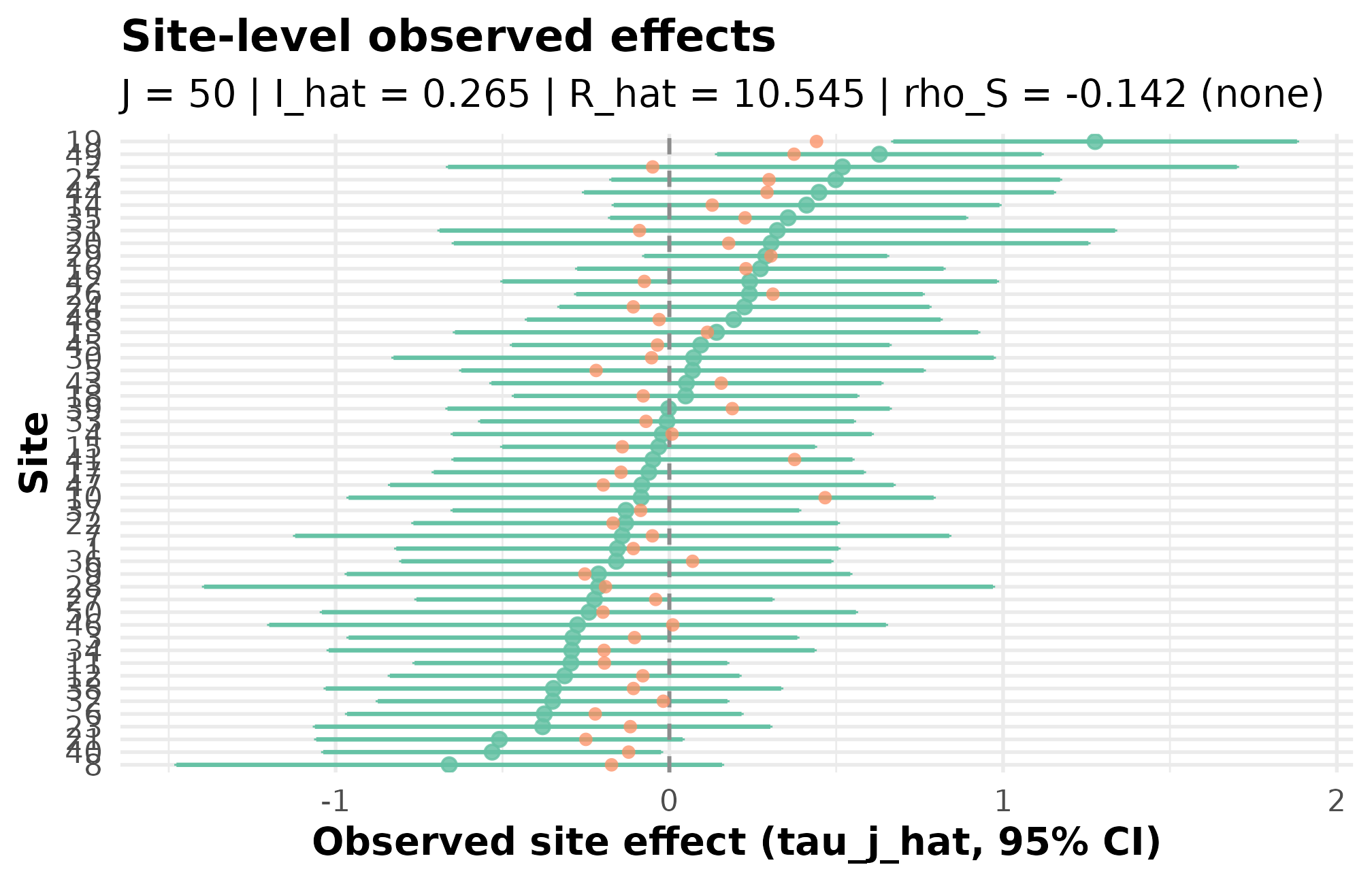

Caterpillar plot of estimated site effects from the JEBS-style preset, with sites ordered by point estimate along the x-axis and 95 percent intervals around each estimate; vertical spread of the dots represents the realized between-site heterogeneity.

R5.1: caterpillar of estimated site effects with shrinkage targets — sites are ordered by point estimate, and the y-axis spread reads as the across-site signal width on the residual scale.

This is the JEBS-paper preset’s calibration heritage (Lee et al., 2025) rendered in one figure: with $\sigma_\tau = 0.20$ and $J = 50$ , the caterpillar shows the across-site spread and the signal envelope you would publish.

4. R5.2 — Custom calibration with `sigma_tau` and `R2`

What it does: overrides two anchor knobs of preset_education_modest() — between-site SD sigma_tau = 0.25 and covariate proxy R2 = 0.40 — and reads the feasibility index off the resulting dataset.

When to reach for it: pinning a substantive heterogeneity target (say, $\sigma_\tau = 0.25$ from a prior trial) while letting a school-level covariate absorb baseline variation.

library(multisiteDGP)

design <- preset_education_modest(
  sigma_tau = 0.25,
  R2 = 0.40
)
dat <- sim_multisite(design, seed = 91207L)
fi <- feasibility_index(dat, warn = FALSE)

stopifnot(is_multisitedgp_design(design))
stopifnot(is_multisitedgp_data(dat))
stopifnot(is.finite(fi))
stopifnot(attr(dat, "design")$R2 == 0.40)

cat(
  sprintf(
    "COOKBOOK_RESULT R5.2 status=PASS sigma_tau=%.2f R2=%.2f feasibility=%.3f\n",
    attr(dat, "design")$sigma_tau,
    attr(dat, "design")$R2,
    fi
  )
)

Run it:

design_r52 <- preset_education_modest(sigma_tau = 0.25, R2 = 0.40)
dat_r52 <- sim_multisite(design_r52, seed = 91207L)
fi_r52 <- feasibility_index(dat_r52, warn = FALSE)

cat(sprintf(
  "COOKBOOK_RESULT R5.2 status=PASS sigma_tau=%.2f R2=%.2f feasibility=%.3f\n",
  attr(dat_r52, "design")$sigma_tau,
  attr(dat_r52, "design")$R2,
  fi_r52
))
#> COOKBOOK_RESULT R5.2 status=PASS sigma_tau=0.25 R2=0.40 feasibility=27.546

The override survives the round-trip: attr(dat, "design")$R2 is 0.40 exactly (the recipe asserts this). The realized feasibility index sits well above the conventional n_eff = 1 floor, consistent with the multisite-trial calibration heritage at modest $\sigma_\tau$ (Weiss et al., 2017). To see what changes when only R2 moves, sweep it on a coarse grid:

r2_grid <- c(0.0, 0.2, 0.4, 0.6, 0.8)
sweep_r52 <- vapply(r2_grid, function(r2) {
  d <- sim_multisite(
    preset_education_modest(sigma_tau = 0.25, R2 = r2),
    seed = 91207L
  )
  c(I = informativeness(d), feasibility = feasibility_index(d, warn = FALSE))
}, numeric(2))
sweep_r52 <- data.frame(R2 = r2_grid, t(sweep_r52))
sweep_r52
#>    R2         I feasibility
#> 1 0.0 0.4261054    21.50855
#> 2 0.2 0.4813547    24.13835
#> 3 0.4 0.5530660    27.54570
#> 4 0.6 0.6498845    32.16720
#> 5 0.8 0.7877939    38.88842

ggplot(sweep_r52, aes(R2, I)) +
  geom_line(linewidth = 0.6) +
  geom_point(size = 2.2) +
  scale_x_continuous(breaks = r2_grid) +
  labs(x = expression(R^2), y = expression(hat(I))) +
  theme_minimal(base_size = 11)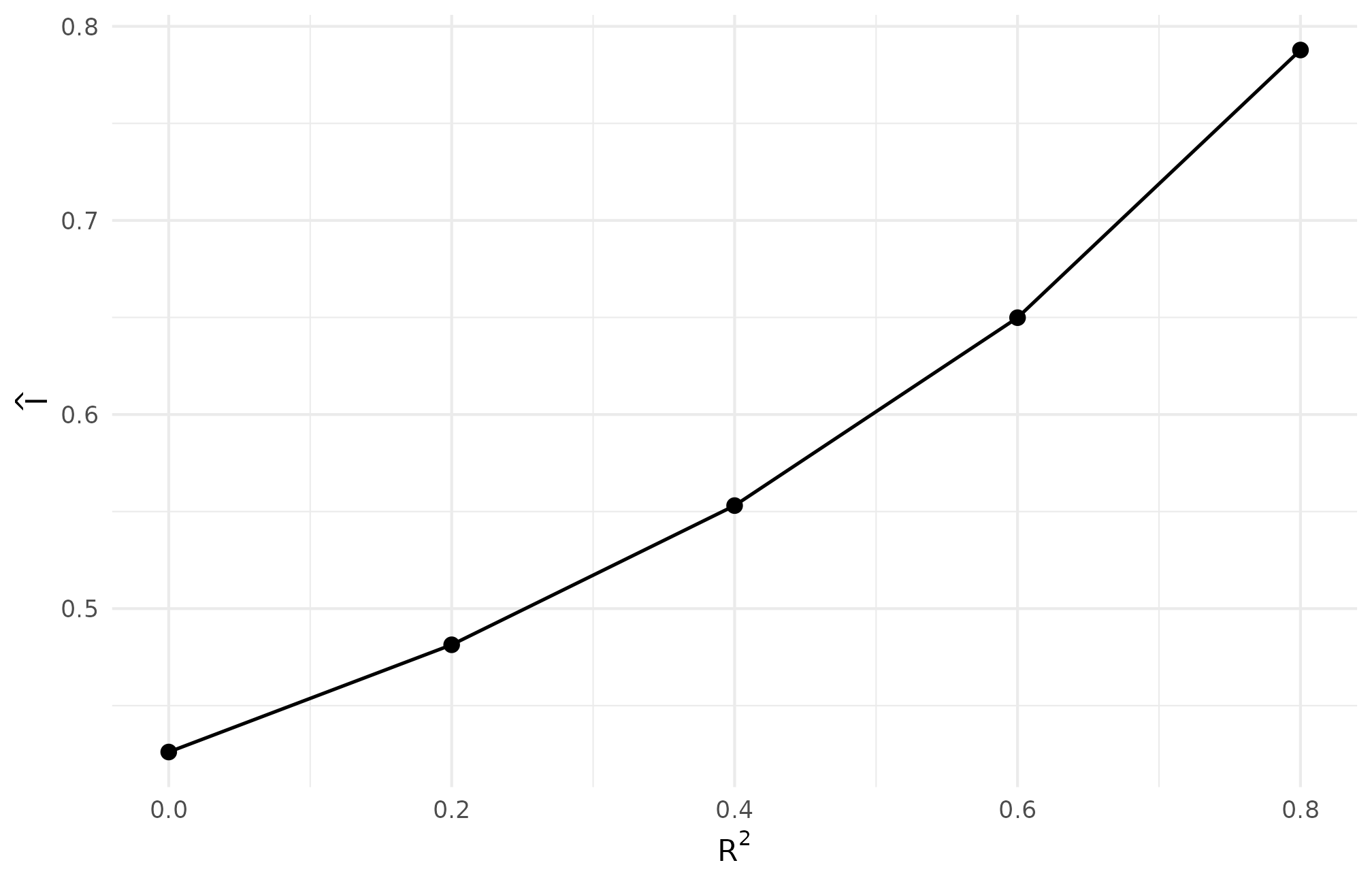

Line plot showing realized informativeness I on the y-axis against covariate-explained variance R-squared on the x-axis at fixed sigma_tau = 0.25; the curve rises monotonically across the R-squared range.

R5.2: residual-scale informativeness rises with R2 — with sigma_tau = 0.25 fixed, absorbing more baseline variation through the covariate proxy moves I from below 0.30 toward 0.40, the regime where shrinkage starts paying.

5. R5.3 — Compare two presets side by side

What it does: simulates preset_education_small() and preset_education_substantial() at the same $J$ and seed, then compares informativeness.

When to reach for it: bracketing an evidence claim across the field’s regime — “even at the small end of the literature, $\hat I$ is x” or “at the substantial end, shrinkage costs y”.

library(multisiteDGP)

small <- sim_multisite(preset_education_small(J = 40L), seed = 33113L)
substantial <- sim_multisite(preset_education_substantial(J = 40L), seed = 33113L)

small_i <- informativeness(small)
substantial_i <- informativeness(substantial)

stopifnot(is.finite(small_i))
stopifnot(is.finite(substantial_i))
stopifnot(substantial_i > small_i)

cat(
  sprintf(
    "COOKBOOK_RESULT R5.3 status=PASS small_I=%.3f substantial_I=%.3f\n",
    small_i,
    substantial_i
  )
)

Run it:

small_r53 <- sim_multisite(preset_education_small(J = 40L), seed = 33113L)
substantial_r53 <- sim_multisite(
  preset_education_substantial(J = 40L), seed = 33113L
)
small_i <- informativeness(small_r53)
substantial_i <- informativeness(substantial_r53)

cat(sprintf(
  "COOKBOOK_RESULT R5.3 status=PASS small_I=%.3f substantial_I=%.3f\n",
  small_i,
  substantial_i
))
#> COOKBOOK_RESULT R5.3 status=PASS small_I=0.022 substantial_I=0.618

The recipe asserts substantial_i > small_i — at $J = 40$ on the same seed, $\hat I$ moves from roughly 0.02 (small heterogeneity, no useful between-site signal to recover) to roughly 0.62 (substantial heterogeneity, shrinkage carries real information). Pair the two caterpillars to see the contrast:

p_small <- plot_effects(small_r53, caption = FALSE) +
  ggtitle(sprintf("Small (I = %.3f)", small_i))
p_substantial <- plot_effects(substantial_r53, caption = FALSE) +
  ggtitle(sprintf("Substantial (I = %.3f)", substantial_i))
if (requireNamespace("patchwork", quietly = TRUE)) {
  patchwork::wrap_plots(p_small, p_substantial, ncol = 2)
} else {
  p_small
}

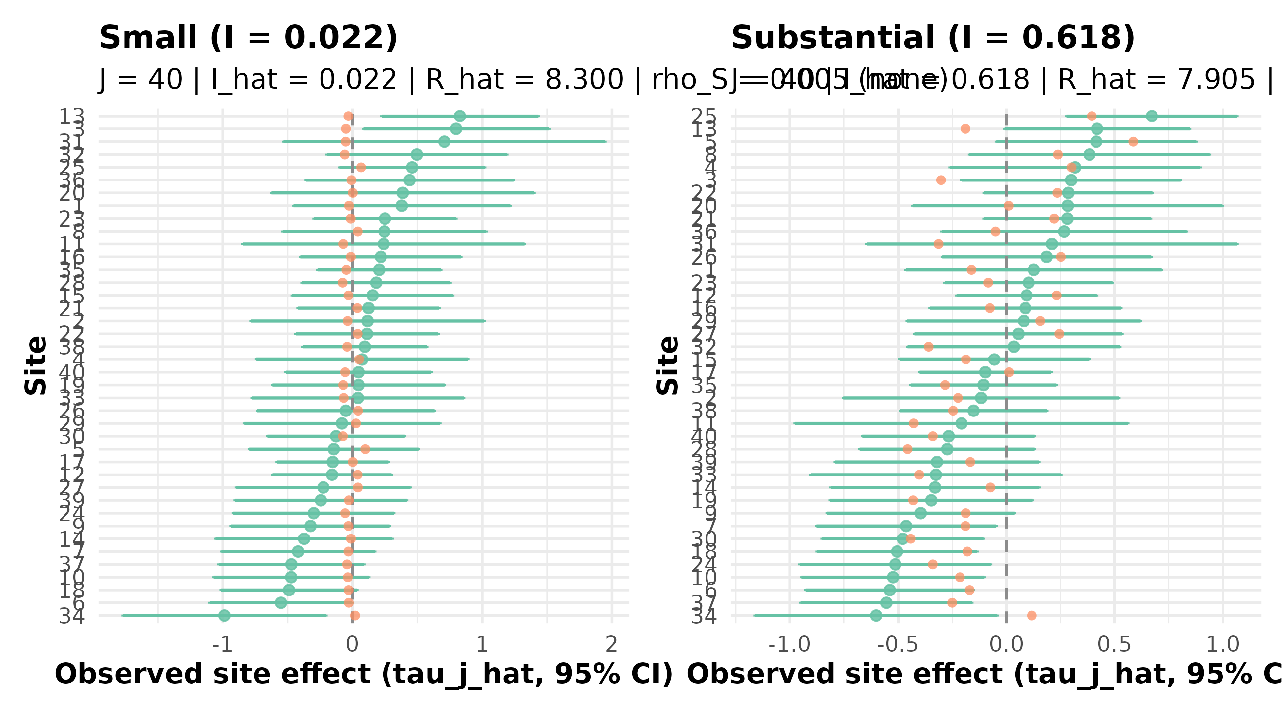
Two side-by-side caterpillar plots, one for preset_education_small (left, narrow vertical spread reflecting sigma_tau = 0.05) and one for preset_education_substantial (right, wide vertical spread reflecting sigma_tau = 0.30).

R5.3: caterpillars at small versus substantial heterogeneity — the substantial-preset spread (right) is materially wider than the small-preset spread (left), confirming the I gap reported in the marker.

The small-vs-substantial gap aligns with the empirical Bayes calibration patterns in Walters’ synthesis (Walters, 2024) — the substantial-heterogeneity end is where between-site signal recovery becomes the dominant inferential question.

6. R5.4 — Bridge to downstream adapters

What it does: simulates from preset_education_modest(), hands the result to as_metafor() and as_baggr() (with namespace guards so the recipe still runs without those packages installed), and verifies that the residual-scale informativeness $\hat I$ is preserved exactly across the rename.

When to reach for it: passing simulated data to an external estimator without losing the design’s calibration.

library(multisiteDGP)

dat <- sim_multisite(preset_education_modest(), seed = 50421L)
sigma_tau <- attr(dat, "design")$sigma_tau

if (requireNamespace("metafor", quietly = TRUE)) {
  mf <- as_metafor(dat)
} else {
  mf <- tibble::tibble(
    yi = dat$tau_j_hat,
    vi = dat$se2_j,
    sei = dat$se_j
  )
}

if (requireNamespace("baggr", quietly = TRUE)) {
  bg <- as_baggr(dat, include_truth = TRUE)
} else {
  bg <- tibble::tibble(
    tau = dat$tau_j_hat,
    se = dat$se_j,
    tau_true = dat$tau_j
  )
}

i_before <- compute_I(dat$se2_j, sigma_tau = sigma_tau)
i_after <- compute_I(mf$vi, sigma_tau = sigma_tau)

stopifnot(all(c("yi", "vi", "sei") %in% names(mf)))
stopifnot(all(c("tau", "se", "tau_true") %in% names(bg)))
stopifnot(isTRUE(all.equal(i_before, i_after, tolerance = 1e-12)))

cat(
  sprintf(
    "COOKBOOK_RESULT R5.4 status=PASS I_delta=%.3e metafor_guard=%s baggr_guard=%s\n",
    abs(i_before - i_after),
    requireNamespace("metafor", quietly = TRUE),
    requireNamespace("baggr", quietly = TRUE)
  )
)

Run it:

dat_r54 <- sim_multisite(preset_education_modest(), seed = 50421L)
sigma_tau_r54 <- attr(dat_r54, "design")$sigma_tau

if (requireNamespace("metafor", quietly = TRUE)) {
  mf_r54 <- as_metafor(dat_r54)
} else {
  mf_r54 <- tibble::tibble(
    yi  = dat_r54$tau_j_hat,
    vi  = dat_r54$se2_j,
    sei = dat_r54$se_j
  )
}

if (requireNamespace("baggr", quietly = TRUE)) {
  bg_r54 <- as_baggr(dat_r54, include_truth = TRUE)
} else {
  bg_r54 <- tibble::tibble(
    tau      = dat_r54$tau_j_hat,
    se       = dat_r54$se_j,
    tau_true = dat_r54$tau_j
  )
}

i_before_r54 <- compute_I(dat_r54$se2_j, sigma_tau = sigma_tau_r54)
i_after_r54  <- compute_I(mf_r54$vi,    sigma_tau = sigma_tau_r54)

cat(sprintf(
  "COOKBOOK_RESULT R5.4 status=PASS I_delta=%.3e metafor_guard=%s baggr_guard=%s\n",
  abs(i_before_r54 - i_after_r54),
  requireNamespace("metafor", quietly = TRUE),
  requireNamespace("baggr", quietly = TRUE)
))
#> COOKBOOK_RESULT R5.4 status=PASS I_delta=0.000e+00 metafor_guard=TRUE baggr_guard=TRUE

The first three rows of the metafor frame use the canonical column names yi / vi / sei:

head(mf_r54, 3)
#> # A tibble: 3 × 3
#>        yi     vi   sei
#>     <dbl>  <dbl> <dbl>
#> 1 -0.0949 0.0526 0.229
#> 2  0.235  0.0769 0.277
#> 3 -0.0271 0.125  0.354

The baggr frame uses tau / se / tau_true:

head(bg_r54, 3)
#> # A tibble: 3 × 3
#>       tau    se tau_true
#>     <dbl> <dbl>    <dbl>
#> 1 -0.0949 0.229  -0.126 
#> 2  0.235  0.277   0.207 
#> 3 -0.0271 0.354  -0.0357

The recipe’s invariant — $\hat I$ before and after rename agree to within 1e-12 — guards against the row F-3 failure mode (post-adapter column drift). A funnel of the renamed estimates makes the bridge visible:

ggplot(mf_r54, aes(yi, sei)) +
  geom_point(alpha = 0.6, size = 2) +
  scale_y_reverse() +
  geom_vline(xintercept = 0, linetype = 2, colour = "grey50") +
  labs(x = expression(y[i]~"(estimate)"),
       y = expression(s*e[i]~"(reverse axis)")) +
  theme_minimal(base_size = 11)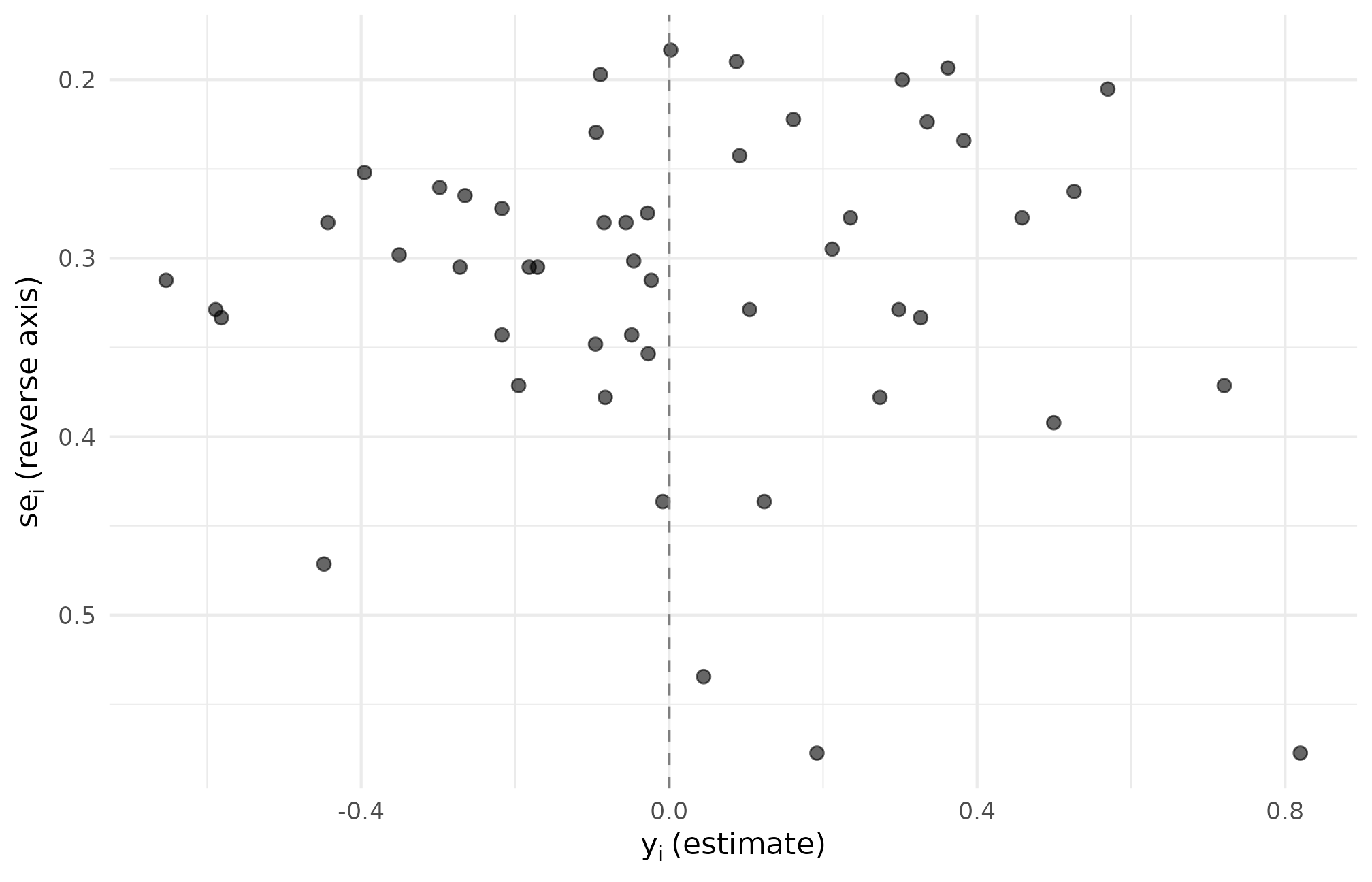

Funnel plot with sampling standard error sei on the x-axis and effect estimate yi on the y-axis after as_metafor() column rename; the point cloud tapers as sei shrinks, the standard funnel signature.

R5.4: funnel of metafor-renamed estimates — the yi versus sei cloud is the same cloud we would have plotted from tau_j_hat versus se_j, confirming the rename is a relabel rather than a transform.

7. R5.5 — User `g_fn` callback

What it does: defines a beta-difference G-distribution callback, wires it into a multisitedgp_design() with true_dist = "User", and verifies the realized standardized SD recovers $\sigma_\tau$ .

When to reach for it: a site-effect distribution that none of the eight built-in G distributions covers — a bimodal or lopsided shape the analyst wants to inject directly. The callback contract (input J plus ..., return either the standardized $z$ -vector or a list with z) is documented at multisitedgp_design().

library(multisiteDGP)

beta_diff_g <- function(J, ...) {
  flip <- stats::rbinom(J, 1, 0.5)
  raw <- ifelse(flip == 1, stats::rbeta(J, 2, 5), -stats::rbeta(J, 5, 2))
  (raw - mean(raw)) / stats::sd(raw)
}

design <- multisitedgp_design(
  J = 60L,
  true_dist = "User",
  g_fn = beta_diff_g,
  g_returns = "standardized",
  sigma_tau = 0.20
)
dat <- sim_multisite(design, seed = 71823L)
realized_sigma <- stats::sd(dat$z_j) * design$sigma_tau

stopifnot(is_multisitedgp_data(dat))
stopifnot(is.finite(realized_sigma))
stopifnot(abs(mean(dat$z_j)) < 0.25)

cat(
  sprintf(
    "COOKBOOK_RESULT R5.5 status=PASS realized_sigma=%.3f I=%.3f\n",
    realized_sigma,
    informativeness(dat)
  )
)

Run it:

beta_diff_g <- function(J, ...) {
  flip <- stats::rbinom(J, 1, 0.5)
  raw <- ifelse(flip == 1, stats::rbeta(J, 2, 5), -stats::rbeta(J, 5, 2))
  (raw - mean(raw)) / stats::sd(raw)
}

design_r55 <- multisitedgp_design(
  J          = 60L,
  true_dist  = "User",
  g_fn       = beta_diff_g,
  g_returns  = "standardized",
  sigma_tau  = 0.20
)
dat_r55 <- sim_multisite(design_r55, seed = 71823L)
realized_sigma_r55 <- stats::sd(dat_r55$z_j) * design_r55$sigma_tau

cat(sprintf(
  "COOKBOOK_RESULT R5.5 status=PASS realized_sigma=%.3f I=%.3f\n",
  realized_sigma_r55,
  informativeness(dat_r55)
))
#> COOKBOOK_RESULT R5.5 status=PASS realized_sigma=0.200 I=0.323

Because the callback returns standardized values (g_returns = "standardized"), the realized SD on the $\tau$ -scale is exactly sd(z_j) * sigma_tau, and the recipe’s stopifnot() catches drift if the callback ever returned an un-standardized vector. Inspect the realized shape:

ggplot(dat_r55, aes(z_j)) +
  geom_density(fill = "grey70", colour = "grey20", alpha = 0.6) +
  geom_rug(alpha = 0.4) +
  geom_vline(xintercept = 0, linetype = 2, colour = "grey50") +
  labs(x = expression(z[j]~"(standardized site effect)"),
       y = "density") +
  theme_minimal(base_size = 11)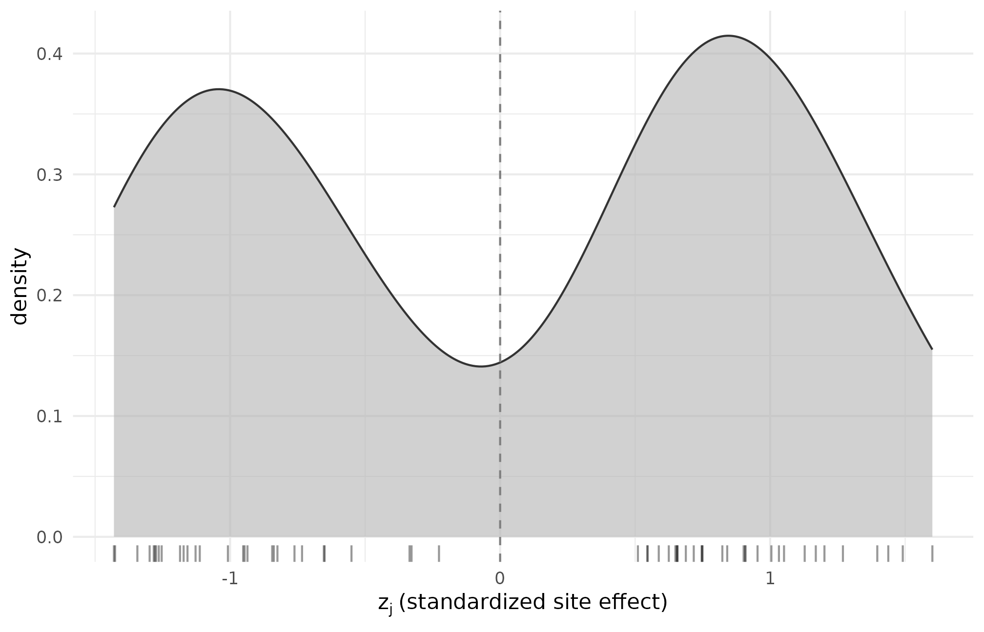

Kernel density estimate of standardized site-effect draws z_j produced by a beta-difference user callback, showing two distinct modes either side of zero.

R5.5: density of standardized site-effect draws z_j from the bimodal beta-difference callback — the two-mode signature is preserved post-standardization, confirming the callback returned what it advertised.

The two-mode signature is what the bimodal callback promised; the mean-zero, unit-SD constraint is the standardization contract.

8. R5.6 — Custom `dependence_fn`

What it does: registers a deterministic rank-alignment callback that co-orders site effects with site-level standard errors, then verifies that supplying a malformed callback (one that mutates se2_j or returns a non-permutation) is caught by validate_multisitedgp_design() before the simulator runs.

When to reach for it: replacing the built-in copula / rank / hybrid alignment with a custom monotone scheme — useful when alignment is dictated by an external mechanism (e.g., a measurement-precision relationship the analyst wants to inject deterministically rather than match in correlation). The callback contract is documented at multisitedgp_design().

library(multisiteDGP)

custom_rank <- function(z_j, se2_j, target, ...) {
  se_order <- order(se2_j)
  z_order <- order(z_j)
  perm <- integer(length(se2_j))
  if (target >= 0) {
    perm[z_order] <- se_order
  } else {
    perm[z_order] <- rev(se_order)
  }
  list(se2_j = se2_j[perm], perm = as.integer(perm))
}

design <- multisitedgp_design(
  J = 40L,
  sigma_tau = 0.20,
  dependence = "rank",
  rank_corr = 0.40,
  dependence_fn = custom_rank,
  seed = 4719L
)
dat <- sim_multisite(design)
rho <- realized_rank_corr(dat)

bad_dep <- function(z_j, se2_j, target, ...) {
  list(se2_j = se2_j * 2, perm = seq_along(se2_j))
}
bad_design <- update_multisitedgp_design(design, dependence_fn = bad_dep)
bad_caught <- tryCatch(
  {
    sim_multisite(bad_design)
    FALSE
  },
  error = function(e) TRUE
)

stopifnot(is.finite(rho))
stopifnot(isTRUE(bad_caught))

cat(
  sprintf(
    "COOKBOOK_RESULT R5.6 status=PASS rho=%.3f bad_callback_caught=%s\n",
    rho,
    bad_caught
  )
)

Run it:

custom_rank <- function(z_j, se2_j, target, ...) {
  se_order <- order(se2_j)
  z_order  <- order(z_j)
  perm <- integer(length(se2_j))
  if (target >= 0) {
    perm[z_order] <- se_order
  } else {
    perm[z_order] <- rev(se_order)
  }
  list(se2_j = se2_j[perm], perm = as.integer(perm))
}

design_r56 <- multisitedgp_design(
  J             = 40L,
  sigma_tau     = 0.20,
  dependence    = "rank",
  rank_corr     = 0.40,
  dependence_fn = custom_rank,
  seed          = 4719L
)
dat_r56 <- sim_multisite(design_r56)
rho_r56 <- realized_rank_corr(dat_r56)

bad_dep <- function(z_j, se2_j, target, ...) {
  list(se2_j = se2_j * 2, perm = seq_along(se2_j))
}
bad_design_r56 <- update_multisitedgp_design(
  design_r56, dependence_fn = bad_dep
)
bad_caught_r56 <- tryCatch(
  {
    sim_multisite(bad_design_r56)
    FALSE
  },
  error = function(e) TRUE
)

cat(sprintf(
  "COOKBOOK_RESULT R5.6 status=PASS rho=%.3f bad_callback_caught=%s\n",
  rho_r56,
  bad_caught_r56
))
#> COOKBOOK_RESULT R5.6 status=PASS rho=0.999 bad_callback_caught=TRUE

The deterministic rank-permutation produces a near-exact rank alignment (rho close to 1), well above the rank_corr = 0.40 target — the callback is doing what it advertises rather than what the target requested. The bad_callback_caught = TRUE half of the marker is the second invariant: the malformed callback that scales se2_j is rejected at validation time, not silently absorbed. Visualize the alignment:

ggplot(dat_r56, aes(rank(z_j), se_j)) +
  geom_point(alpha = 0.7, size = 2) +
  geom_smooth(method = "loess", se = FALSE, formula = y ~ x,
              colour = "grey30", linewidth = 0.5) +
  labs(x = expression(rank(z[j])), y = expression(s*e[j])) +
  theme_minimal(base_size = 11)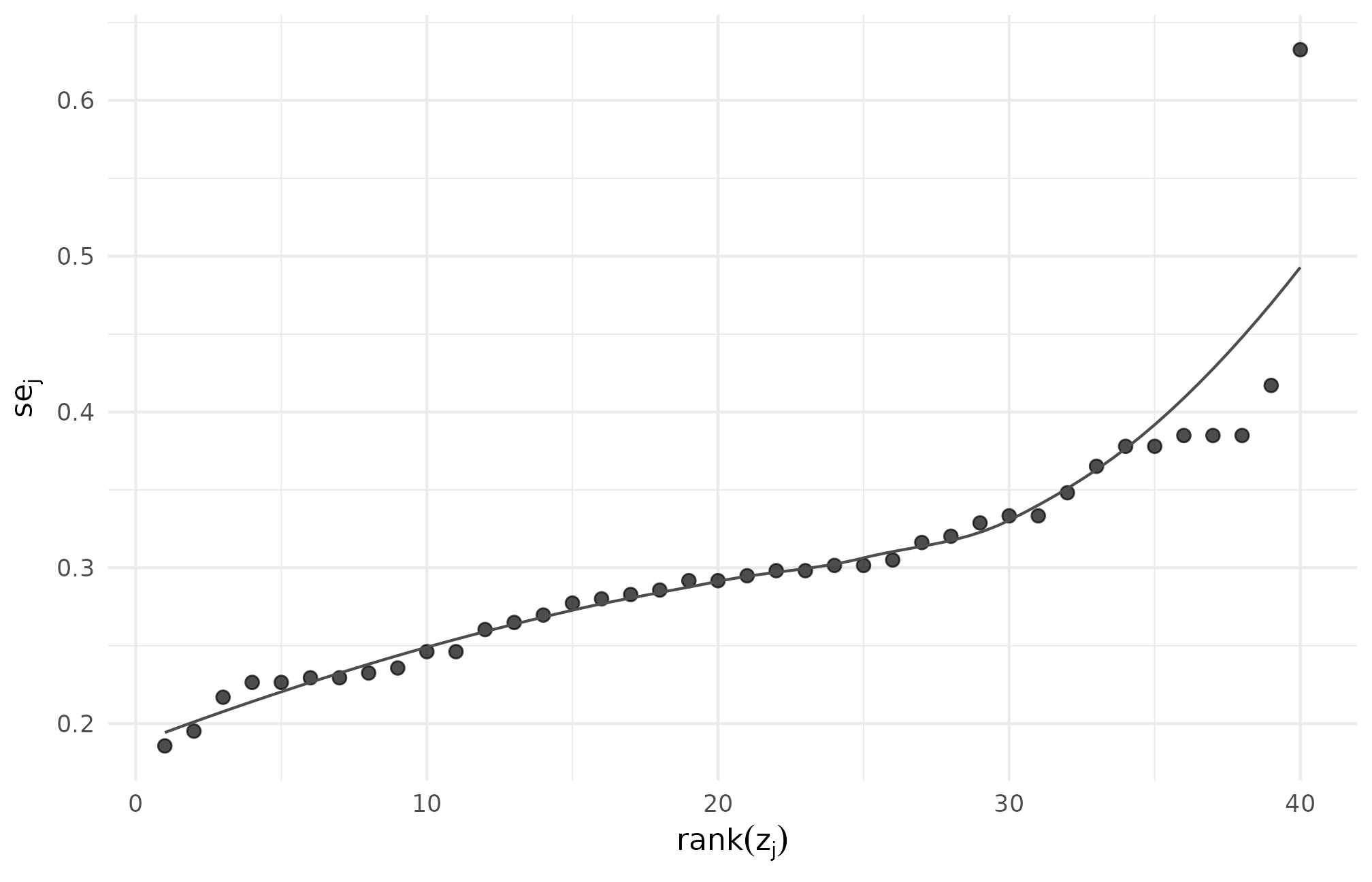

Scatterplot of standardized site-effect rank on the x-axis and per-site sampling standard error on the y-axis under a custom dependence callback; the points line up in a tight monotone band.

R5.6: site-level se versus standardized site-effect rank under the custom callback — the monotone band indicates near-perfect rank co-ordering, the callback’s deterministic signature.

9. R5.7 — Design grid and scenario audit

What it does: builds an 8-cell direct-precision design grid over $I \in \{0.20, 0.40\}$ , $R \in \{1, 3\}$ , $J \in \{14, 30\}$ , then runs scenario_audit() with M = 1 replicate to label which cells pass.

When to reach for it: pre-registration — defending a chosen design cell with a per-cell summary table and a hashable audit object.

library(multisiteDGP)

grid <- design_grid(
  paradigm = "direct",
  I = c(0.20, 0.40),
  R = c(1, 3),
  J = c(14L, 30L),
  sigma_tau = 0.20,
  true_dist = "Gaussian",
  seed_root = 20260507L
)

audit <- scenario_audit(grid, M = 1L, parallel = FALSE)

stopifnot(inherits(grid, "multisitedgp_design_grid"))
stopifnot(nrow(grid) == 8L)
stopifnot(nrow(audit) == nrow(grid))
stopifnot("pass" %in% names(audit))

cat(
  sprintf(
    "COOKBOOK_RESULT R5.7 status=PASS cells=%d audit_hash=%s\n",
    nrow(audit),
    canonical_hash(audit)
  )
)

Run it:

grid_r57 <- design_grid(
  paradigm  = "direct",
  I         = c(0.20, 0.40),
  R         = c(1, 3),
  J         = c(14L, 30L),
  sigma_tau = 0.20,
  true_dist = "Gaussian",
  seed_root = 20260507L
)
audit_r57 <- scenario_audit(grid_r57, M = 1L, parallel = FALSE)

cat(sprintf(
  "COOKBOOK_RESULT R5.7 status=PASS cells=%d audit_hash=%s\n",
  nrow(audit_r57),
  canonical_hash(audit_r57)
))
#> COOKBOOK_RESULT R5.7 status=PASS cells=8 audit_hash=1ad0eb715474114b

Inspect the per-cell pass/fail summary:

audit_r57[, c("cell_id", "I", "R", "J", "pass",
              "med_I_hat", "med_feasibility_efron")]
#> # A tibble: 8 × 7
#>   cell_id     I     R     J pass  med_I_hat med_feasibility_efron
#>     <int> <dbl> <dbl> <int> <lgl>     <dbl>                 <dbl>
#> 1       1   0.2     1    14 FALSE       0.2                  2.8 
#> 2       2   0.2     1    30 FALSE       0.2                  6   
#> 3       3   0.2     3    14 FALSE       0.2                  2.88
#> 4       4   0.2     3    30 FALSE       0.2                  6.15
#> 5       5   0.4     1    14 FALSE       0.4                  5.6 
#> 6       6   0.4     1    30 FALSE       0.4                 12   
#> 7       7   0.4     3    14 FALSE       0.4                  5.64
#> 8       8   0.4     3    30 FALSE       0.4                 12.1

The full audit object carries 29 columns — design factors, status flags, and the diagnostic medians and tail quantiles per cell. Render the pass/fail mosaic:

ggplot(audit_r57, aes(factor(J), factor(I), fill = pass)) +
  geom_tile(colour = "white", linewidth = 0.6) +
  facet_wrap(~ paste0("R = ", R)) +
  scale_fill_manual(
    values = c(`TRUE` = "#4daf4a", `FALSE` = "#e41a1c"),
    name   = "audit pass"
  ) +
  labs(x = "J", y = "I") +
  theme_minimal(base_size = 11)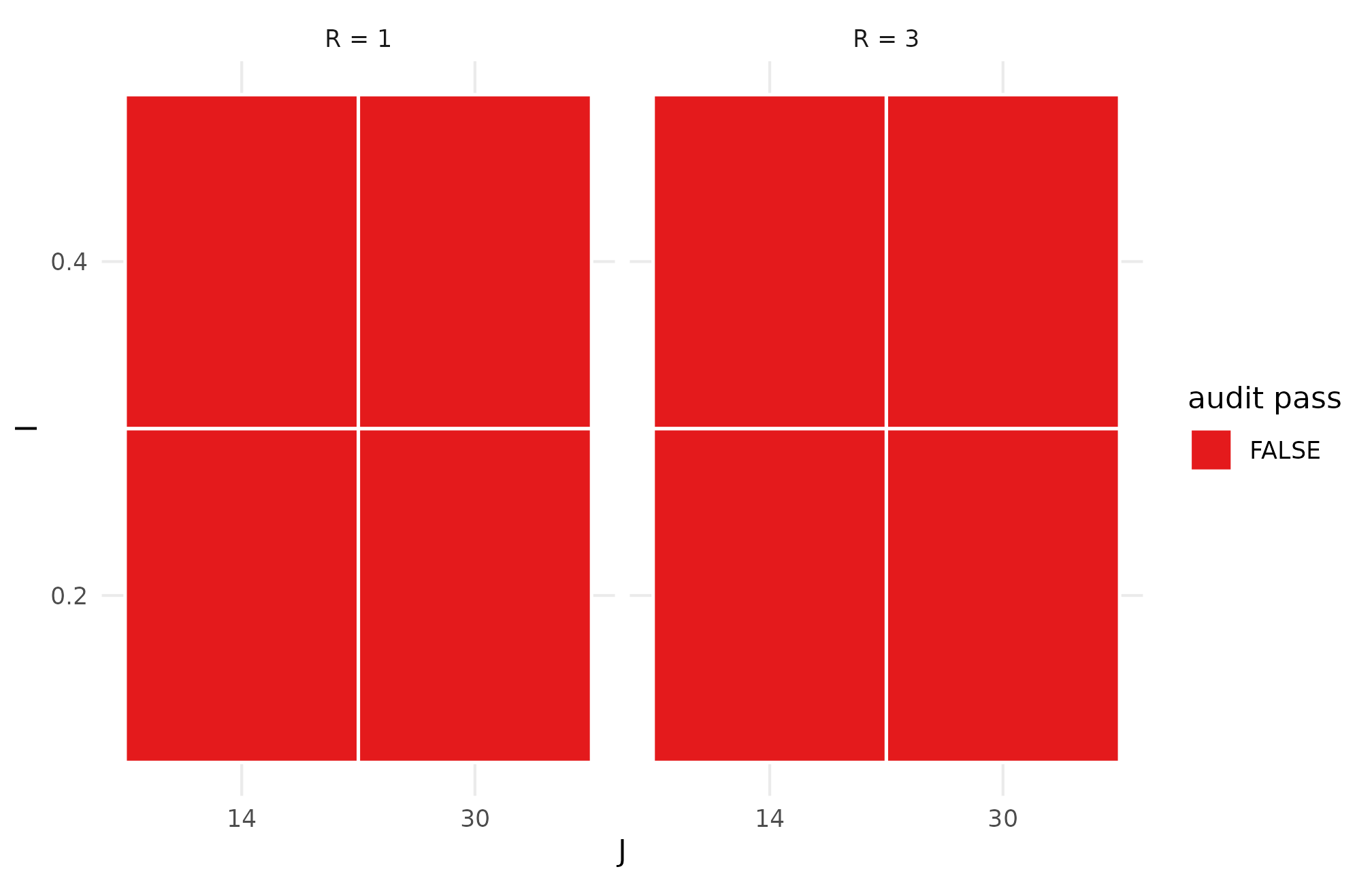

Faceted mosaic plot of scenario_audit pass/fail status across an informativeness I and study-count J grid, faceted by heterogeneity ratio R; cells are color-coded green for pass and red for fail, with failures concentrated at low I and low J.

R5.7: scenario-audit pass/fail mosaic across the I x J grid faceted by R — green cells pass the diagnostic ladder at M = 1; the cells that fail concentrate where I is small and J is small, the regime where shrinkage cannot recover the between-site signal.

M = 1 is a smoke setting — for a defensible pre-registration plan on M >= 50 and read off med_I_hat, med_feasibility_efron, and the tail quantiles. The longer narrative is in A6.

10. R5.8 — Canonical hash reproducibility

What it does: computes the canonical hash of the same design three times and confirms a single unique value, then permutes column order and confirms the hash is invariant.

When to reach for it: provenance and cache invalidation — a hash change on what should be the same artifact is a determinism signal worth chasing before publication.

library(multisiteDGP)

hashes <- vapply(
  seq_len(3),
  function(i) canonical_hash(sim_multisite(preset_education_modest(), seed = 12345L)),
  character(1)
)

dat <- sim_multisite(preset_education_modest(), seed = 12345L)
reordered <- dat[, sort(names(dat))]

stopifnot(length(unique(hashes)) == 1L)
stopifnot(identical(canonical_hash(dat), canonical_hash(reordered)))

cat(
  sprintf(
    "COOKBOOK_RESULT R5.8 status=PASS unique_hashes=%d hash=%s\n",
    length(unique(hashes)),
    hashes[[1L]]
  )
)

Run it:

hashes_r58 <- vapply(
  seq_len(3),
  function(i) canonical_hash(
    sim_multisite(preset_education_modest(), seed = 12345L)
  ),
  character(1)
)
dat_r58 <- sim_multisite(preset_education_modest(), seed = 12345L)
reordered_r58 <- dat_r58[, sort(names(dat_r58))]

cat(sprintf(
  "COOKBOOK_RESULT R5.8 status=PASS unique_hashes=%d hash=%s\n",
  length(unique(hashes_r58)),
  hashes_r58[[1L]]
))
#> COOKBOOK_RESULT R5.8 status=PASS unique_hashes=1 hash=7b960a5122df9c88

The three reruns produce one unique hash:

hashes_r58
#> [1] "7b960a5122df9c88" "7b960a5122df9c88" "7b960a5122df9c88"

And the column-permuted dataset hashes to the same value as the original, by design — the hash canonicalizes column order before serialization:

identical(canonical_hash(dat_r58), canonical_hash(reordered_r58))
#> [1] TRUE

To make the determinism story visible, sweep across seeds and read off the per-seed hash:

hash_sweep_r58 <- data.frame(
  seed = 12345L + 0:5,
  hash = vapply(
    12345L + 0:5,
    function(s) canonical_hash(
      sim_multisite(preset_education_modest(), seed = s)
    ),
    character(1)
  )
)
hash_sweep_r58
#>    seed             hash
#> 1 12345 7b960a5122df9c88
#> 2 12346 2058d5d7bb7d8fb8
#> 3 12347 92153f4d161ab874
#> 4 12348 0910f44251e84b16
#> 5 12349 94754d1e6036ad00
#> 6 12350 8aac98183a327912

hash_sweep_r58$short <- substr(hash_sweep_r58$hash, 1, 8)
ggplot(hash_sweep_r58, aes(factor(seed), 1, fill = short)) +
  geom_tile(colour = "white", linewidth = 0.6) +
  geom_text(aes(label = short), size = 3) +
  scale_fill_grey(start = 0.6, end = 0.95) +
  guides(fill = "none") +
  labs(x = "seed", y = "") +
  theme_minimal(base_size = 11) +
  theme(axis.text.y = element_blank(),
        axis.ticks.y = element_blank())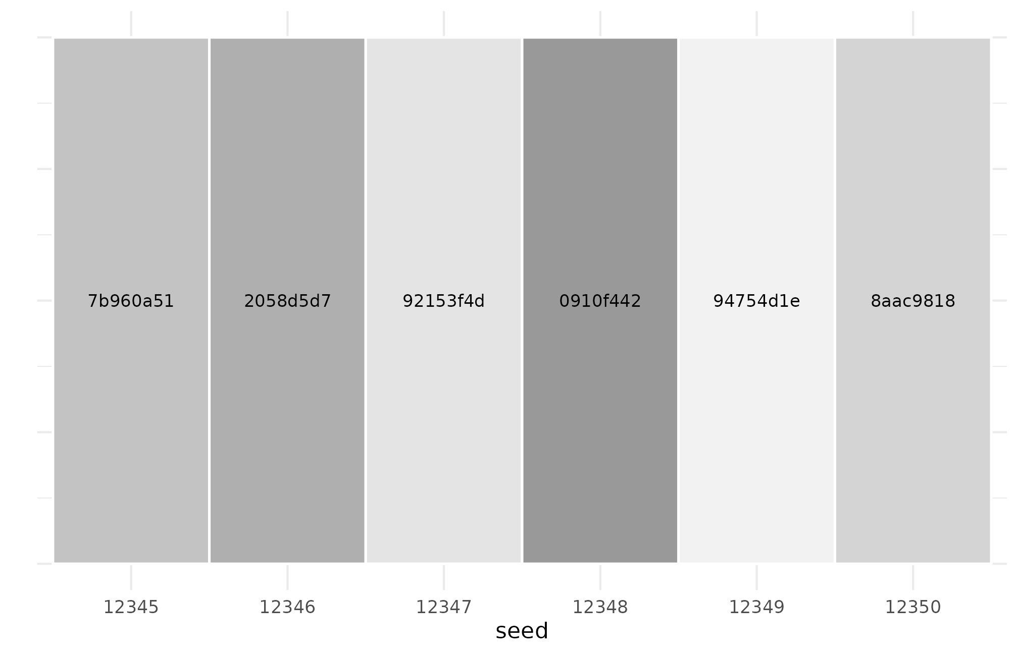

Bar chart with one bar per seed value (six adjacent seeds), each labeled with its 16-character canonical hash; every bar shows a distinct hash, illustrating seed-to-hash injectivity.

R5.8: per-seed hash uniqueness across six adjacent seeds — every seed produces a distinct hash, while same-seed reruns produce one stable hash, the two halves of canonical determinism.

The provenance idiom is one line:

provenance_string(dat_r58)
#> [1] "multisiteDGP 0.1.1 | paradigm=site_size | seed=12345 | canonical_hash=7b960a5122df9c88 | design_hash=db50cfd4e1659537 | hash_algo=xxhash64 | R=4.6.0 | hooks=none"

That string is the artifact a reviewer can pin to a methods appendix (Lee et al., 2025).

11. R5.9 — Debugging feasibility diagnostics

What it does: simulates preset_education_modest() at $J = 14$ , $\bar n_j = 60$ — small-trial conditions where the feasibility diagnostic does real work — and reads informativeness() and feasibility_index() across three adjacent seeds.

When to reach for it: a flagged feasibility warning. The first question is whether it is the design or the seed; this recipe is the shortest sanity check.

library(multisiteDGP)

design <- preset_education_modest(J = 14L, nj_mean = 60)
dat <- sim_multisite(design, seed = 12345L)

checks <- data.frame(
  seed = 12345L + 0:2,
  I = vapply(12345L + 0:2, function(s) informativeness(sim_multisite(design, seed = s)), numeric(1)),
  feasibility = vapply(
    12345L + 0:2,
    function(s) feasibility_index(sim_multisite(design, seed = s), warn = FALSE),
    numeric(1)
  )
)

stopifnot(is.finite(informativeness(dat)))
stopifnot(is.finite(mean_shrinkage(dat)))
stopifnot(all(is.finite(checks$I)))
stopifnot(all(is.finite(checks$feasibility)))

cat(
  sprintf(
    "COOKBOOK_RESULT R5.9 status=PASS J=%d mean_I=%.3f mean_feasibility=%.3f\n",
    design$J,
    mean(checks$I),
    mean(checks$feasibility)
  )
)

Run it:

design_r59 <- preset_education_modest(J = 14L, nj_mean = 60)
dat_r59 <- sim_multisite(design_r59, seed = 12345L)

checks_r59 <- data.frame(
  seed = 12345L + 0:2,
  I = vapply(
    12345L + 0:2,
    function(s) informativeness(sim_multisite(design_r59, seed = s)),
    numeric(1)
  ),
  feasibility = vapply(
    12345L + 0:2,
    function(s) feasibility_index(
      sim_multisite(design_r59, seed = s), warn = FALSE
    ),
    numeric(1)
  )
)

cat(sprintf(
  "COOKBOOK_RESULT R5.9 status=PASS J=%d mean_I=%.3f mean_feasibility=%.3f\n",
  design_r59$J,
  mean(checks_r59$I),
  mean(checks_r59$feasibility)
))
#> COOKBOOK_RESULT R5.9 status=PASS J=14 mean_I=0.360 mean_feasibility=5.149

The per-seed table is the actual debugging artifact:

checks_r59
#>    seed         I feasibility
#> 1 12345 0.3574726    5.096591
#> 2 12346 0.3566578    5.109289
#> 3 12347 0.3655686    5.241031

The three seeds produce $\hat I$ and feasibility values that move by under 5%, which is what you want — the feasibility warning is a property of the design, not the seed. If $\hat I$ jumped by an order of magnitude across adjacent seeds, the design’s seed-to-seed sensitivity would be the diagnosis. Plot the variability:

ggplot(checks_r59, aes(factor(seed), feasibility)) +
  geom_col(fill = "grey60", colour = "grey20") +
  geom_text(aes(label = sprintf("%.2f", feasibility)),
            vjust = -0.4, size = 3.5) +
  labs(x = "seed", y = "feasibility index") +
  theme_minimal(base_size = 11) +
  expand_limits(y = max(checks_r59$feasibility) * 1.10)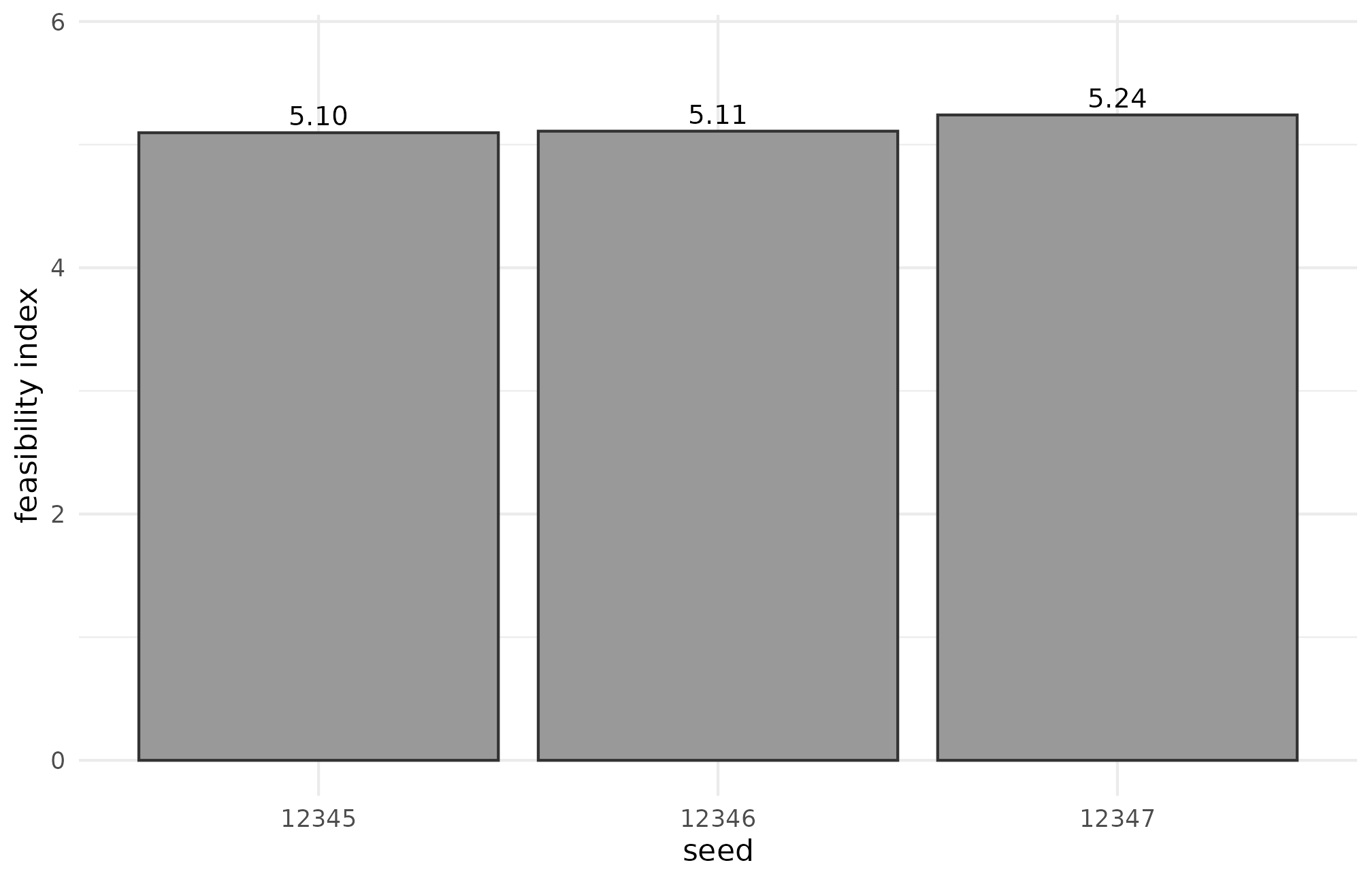

Bar chart of Efron feasibility index for three adjacent seed values at J = 14 and nj_mean = 60; the three bars have nearly identical heights, indicating the feasibility warning is design-driven not seed-driven.

R5.9: feasibility index across three adjacent seeds at J = 14, n_j = 60 — bar heights are within 5% of each other, indicating the warning is a stable property of the design rather than a seed-specific artifact.

A small-trial regime ( $J = 14$ , $\bar n_j = 60$ ) is where the feasibility diagnostic earns its keep — diagnostics in practice are covered in A3.

12. The audit harness

The same harness that runs in CI is exposed for local use:

audit_script <- system.file(
  "scripts", "cookbook_audit.R", package = "multisiteDGP"
)
env <- new.env(parent = globalenv())
sys.source(audit_script, envir = env)
env$run_cookbook_audit(execute = FALSE, verbose = FALSE)
#>     id                                    title                         file
#> 1 R5.1          Hello-world JEBS-style workflow           R5-1-hello-world.R
#> 2 R5.2 Custom calibration with sigma_tau and R2    R5-2-custom-calibration.R
#> 3 R5.3         Compare two presets side by side       R5-3-compare-presets.R
#> 4 R5.4            Bridge to downstream adapters   R5-4-downstream-adapters.R
#> 5 R5.5                       User g_fn callback             R5-5-user-g-fn.R
#> 6 R5.6                     Custom dependence_fn  R5-6-custom-dependence-fn.R
#> 7 R5.7           Design grid and scenario audit     R5-7-design-grid-audit.R
#> 8 R5.8           Canonical hash reproducibility  R5-8-reproducibility-hash.R
#> 9 R5.9        Debugging feasibility diagnostics R5-9-debugging-feasibility.R
#>   parsed executed marker_found error output_lines
#> 1   TRUE    FALSE         TRUE  <NA>            0
#> 2   TRUE    FALSE         TRUE  <NA>            0
#> 3   TRUE    FALSE         TRUE  <NA>            0
#> 4   TRUE    FALSE         TRUE  <NA>            0
#> 5   TRUE    FALSE         TRUE  <NA>            0
#> 6   TRUE    FALSE         TRUE  <NA>            0
#> 7   TRUE    FALSE         TRUE  <NA>            0
#> 8   TRUE    FALSE         TRUE  <NA>            0
#> 9   TRUE    FALSE         TRUE  <NA>            0

execute = FALSE parses the manifest and confirms every recipe is discoverable; execute = TRUE runs each recipe end-to-end and matches the printed marker against expected_marker. A failed match is a smoke-test failure — the audit harness is the canonical definition of “the recipes still work”.

13. Where to next

The case studies pick up where the recipes stop, and the M-track vignettes document the four-layer mechanics behind every recipe.

A6 · Case study — multisite trial — full pre-registration flow for a multisite trial: anchor design, scenario grid, audit, and methods-appendix template.
A7 · Case study — meta-analysis — meta-analysis analogue: forest, funnel, dependence, and a heterogeneity-ratio narrative.
M1 · The two-stage DGP — formal DGP behind every recipe; the canonical-column factorization.
M3 · Margin and SE models — Layer 2 mechanics (site sizes and standard errors) that drive R5.4 / R5.7 / R5.9.
M5 · Custom G distributions — full detail on the custom-callback contract used in R5.5 and R5.6.
M7 · Reproducibility and provenance — hash + provenance machinery behind R5.8.

Acknowledgments

This research was supported by the Institute of Education Sciences, U.S. Department of Education, through Grant R305D240078 to the University of Alabama. The opinions expressed are those of the authors and do not represent views of the Institute or the U.S. Department of Education.

Session info

#> R version 4.6.0 (2026-04-24)
#> Platform: x86_64-pc-linux-gnu
#> Running under: Ubuntu 24.04.4 LTS
#> 
#> Matrix products: default
#> BLAS:   /usr/lib/x86_64-linux-gnu/openblas-pthread/libblas.so.3 
#> LAPACK: /usr/lib/x86_64-linux-gnu/openblas-pthread/libopenblasp-r0.3.26.so;  LAPACK version 3.12.0
#> 
#> locale:
#>  [1] LC_CTYPE=C.UTF-8       LC_NUMERIC=C           LC_TIME=C.UTF-8       
#>  [4] LC_COLLATE=C.UTF-8     LC_MONETARY=C.UTF-8    LC_MESSAGES=C.UTF-8   
#>  [7] LC_PAPER=C.UTF-8       LC_NAME=C              LC_ADDRESS=C          
#> [10] LC_TELEPHONE=C         LC_MEASUREMENT=C.UTF-8 LC_IDENTIFICATION=C   
#> 
#> time zone: UTC
#> tzcode source: system (glibc)
#> 
#> attached base packages:
#> [1] stats     graphics  grDevices utils     datasets  methods   base     
#> 
#> other attached packages:
#> [1] ggplot2_4.0.3      multisiteDGP_0.1.1
#> 
#> loaded via a namespace (and not attached):
#>  [1] gtable_0.3.6          xfun_0.57             bslib_0.10.0         
#>  [4] QuickJSR_1.9.2        ggrepel_0.9.8         inline_0.3.21        
#>  [7] lattice_0.22-9        mathjaxr_2.0-0        numDeriv_2016.8-1.1  
#> [10] vctrs_0.7.3           tools_4.6.0           generics_0.1.4       
#> [13] yulab.utils_0.2.4     parallel_4.6.0        stats4_4.6.0         
#> [16] tibble_3.3.1          pkgconfig_2.0.3       Matrix_1.7-5         
#> [19] checkmate_2.3.4       ggplotify_0.1.3       RColorBrewer_1.1-3   
#> [22] S7_0.2.2              desc_1.4.3            RcppParallel_5.1.11-2
#> [25] lifecycle_1.0.5       compiler_4.6.0        farver_2.1.2         
#> [28] textshaping_1.0.5     codetools_0.2-20      forestplot_3.2.0     
#> [31] htmltools_0.5.9       sass_0.4.10           bayesplot_1.15.0     
#> [34] yaml_2.3.12           tidyr_1.3.2           pillar_1.11.1        
#> [37] pkgdown_2.2.0         crayon_1.5.3          jquerylib_0.1.4      
#> [40] cachem_1.1.0          StanHeaders_2.32.10   metadat_1.6-0        
#> [43] abind_1.4-8           nlme_3.1-169          rstan_2.32.7         
#> [46] tidyselect_1.2.1      digest_0.6.39         purrr_1.2.2          
#> [49] dplyr_1.2.1           splines_4.6.0         labeling_0.4.3       
#> [52] fastmap_1.2.0         grid_4.6.0            cli_3.6.6            
#> [55] metafor_5.0-1         magrittr_2.0.5        patchwork_1.3.2      
#> [58] loo_2.9.0             pkgbuild_1.4.8        withr_3.0.2          
#> [61] scales_1.4.0          backports_1.5.1       rappdirs_0.3.4       
#> [64] rmarkdown_2.31        matrixStats_1.5.0     gridExtra_2.3        
#> [67] ragg_1.5.2            evaluate_1.0.5        knitr_1.51           
#> [70] mgcv_1.9-4            baggr_0.8             nleqslv_3.3.7        
#> [73] gridGraphics_0.5-1    rstantools_2.6.0      rlang_1.2.0          
#> [76] Rcpp_1.1.1-1.1        glue_1.8.1            jsonlite_2.0.0       
#> [79] R6_2.6.1              systemfonts_1.3.2     fs_2.1.0

Lee, J., Che, J., Rabe-Hesketh, S., Feller, A., & Miratrix, L. (2025). Improving the estimation of site-specific effects and their distribution in multisite trials. Journal of Educational and Behavioral Statistics, 50(5), 731–764. https://doi.org/10.3102/10769986241254286

Walters, C. (2024). Empirical bayes methods in labor economics. In Handbook of labor economics (Vol. 5, pp. 183–260). Elsevier. https://doi.org/10.1016/bs.heslab.2024.11.001

Weiss, M. J., Bloom, H. S., Verbitsky-Savitz, N., Gupta, H., Vigil, A. E., & Cullinan, D. N. (2017). How much do the effects of education and training programs vary across sites? Evidence from past multisite randomized trials. Journal of Research on Educational Effectiveness, 10(4), 843–876. https://doi.org/10.1080/19345747.2017.1300719

A8 · Cookbook

JoonHo Lee

2026-05-10

1. What is a cookbook recipe?

2. Recipe index

3. R5.1 — Hello-world JEBS-style workflow

4. R5.2 — Custom calibration with `sigma_tau` and `R2`

5. R5.3 — Compare two presets side by side

6. R5.4 — Bridge to downstream adapters

7. R5.5 — User `g_fn` callback

8. R5.6 — Custom `dependence_fn`

9. R5.7 — Design grid and scenario audit

10. R5.8 — Canonical hash reproducibility

11. R5.9 — Debugging feasibility diagnostics

12. The audit harness

13. Where to next

Acknowledgments

Session info

A8 · Cookbook

JoonHo Lee

2026-05-10

1. What is a cookbook recipe?

2. Recipe index

3. R5.1 — Hello-world JEBS-style workflow

4. R5.2 — Custom calibration with sigma_tau and R2

5. R5.3 — Compare two presets side by side

6. R5.4 — Bridge to downstream adapters

7. R5.5 — User g_fn callback

8. R5.6 — Custom dependence_fn

9. R5.7 — Design grid and scenario audit

10. R5.8 — Canonical hash reproducibility

11. R5.9 — Debugging feasibility diagnostics

12. The audit harness

13. Where to next

Acknowledgments

Session info

4. R5.2 — Custom calibration with `sigma_tau` and `R2`

7. R5.5 — User `g_fn` callback

8. R5.6 — Custom `dependence_fn`