A1 · Getting started — your first multisite simulation • multisiteDGP

Abstract

For researchers designing or evaluating a multisite trial who need a defensible synthetic dataset before real data exist. This vignette walks through one preset call, one sim_multisite() call, and the diagnostic readout that tells you whether the realized design hit its targets. You leave with a 50-site simulation tibble, a caterpillar and funnel plot, and a provenance string suitable for a grant appendix or manuscript caption.

Here is what you will produce in five minutes — a labeled view of 50 simulated school effects, ranked from most-shrunk on the left to least-shrunk on the right, with each site’s 95 percent interval drawn around its observed estimate.

Caterpillar plot of 50 simulated site effects from preset_jebs_paper, with 95 percent intervals drawn around each observed estimate.

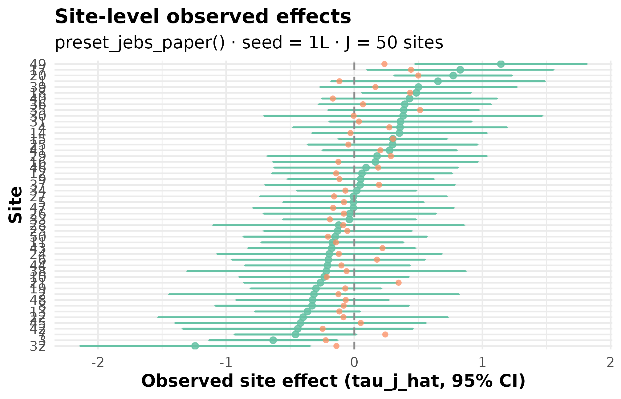
What you will produce in 5 minutes — every dot is a simulated school’s effect estimate; ranked from most-shrunk to least.

Every dot above is a single simulated school. The vertical spread is the heterogeneity the design encodes; the bar widths are the sampling-error structure; the rank order is what your downstream shrinkage estimator will see. The remainder of this vignette walks you through producing the same plot from scratch — and reading the diagnostics that justify trusting it.

1. Why you are here

Maya is writing a grant proposal for a multisite tutoring trial across roughly 50 schools, and the reviewers want to see that her power calculation holds up when between-site heterogeneity is around $\sigma_\tau = 0.20$ . She does not have data yet — she needs a defensible synthetic dataset that mirrors the design she is proposing, plus a one-line provenance string she can drop in the methods appendix.

2. What you will leave with

A 50-site simulated dataset with the canonical columns site_index, z_j, tau_j, tau_j_hat, se_j, se2_j, n_j.
A diagnostic readout that compares realized values against the design’s targets and flags PASS / WARN / FAIL.
Two plots — a caterpillar and a funnel — that make the realized heterogeneity and precision pattern legible at a glance.
A reproducible provenance string carrying a 16-character canonical hash, suitable for a grant appendix or manuscript caption.

3. Install and load

# install.packages("remotes")
remotes::install_github("joonho112/multisiteDGP")

library(multisiteDGP)
library(ggplot2)

The setup chunk above already loaded both, with set.seed(1L). Every primary call below also passes seed = 1L so your local re-run matches the rendered vignette exactly.

4. Your first simulation

Two calls. First, pick a preset — a small, defensible bundle of design parameters tied to a specific scientific scenario. Maya picks preset_jebs_paper() because it matches the JEBS-paper calibration (Lee et al., 2025): $J = 50$ sites, $\sigma_\tau = 0.20$ , mixture-shape latent effects, no induced precision–effect dependence, site sizes drawn around $\bar{n}_j = 40$ .

design <- preset_jebs_paper()
design
#> <multisitedgp_design>
#> Paradigm: site_size    Engine: A1_legacy    Framing: superpopulation
#> J: 50    Seed: NULL (active RNG)    Lifecycle: experimental
#> 
#> [ Layer 1: G-effects ]
#>   true_dist:  Mixture
#>   tau:        0
#>   sigma_tau:  0.2
#>   formula:    NULL
#>   beta:       NULL
#>   g_fn:       NULL
#> 
#> [ Layer 2: Margin (Paradigm A) ]
#>   nj_mean:    40
#>   cv:         0.5
#>   nj_min:     5
#>   p:          0.5
#>   R2:         0
#>   var_outcome: 1
#> 
#> [ Layer 3: Dependence ]
#>   method:        none
#>   rank_corr:     0
#>   pearson_corr:  0
#>   hybrid_init:   copula
#>   hybrid_polish: hill_climb
#>   dependence_fn: NULL
#> 
#> [ Layer 4: Observation ]
#>   obs_fn: NULL
#> 
#> Use sim_multisite(design) or sim_meta(design) to simulate.

Read the printed object as four generative layers. Layer 1 (G-effects) sets the latent shape and the between-site SD. Layer 2 (Margin) controls site sizes and how their sampling variances are produced — this preset uses the site-size-driven path (Paradigm A in the package’s underlying blueprint), where $\widehat{se}_j$ is generated from $n_j$ rather than supplied directly. Layer 3 (Dependence) is set to none. Layer 4 (Observation) adds sampling noise to the latent effect. The design is immutable; to change a field, call update_multisitedgp_design() or pass an override at the multisitedgp_design() constructor.

Now simulate.

dat <- sim_multisite(design, seed = 1L)
dat
#> # A multisitedgp_data: 50 sites, paradigm = "site_size"
#> # Realized vs intended:
#> #   I: realized=0.250 (no target)
#> #   R: realized=7.583 (no target)
#> #   sigma_tau: target=0.200, realized=0.207, PASS
#> #   rho_S: target=0.000, realized=-0.193, PASS
#> #   rho_S_marg: realized=-0.193 (no target)
#> #   Feasibility: WARN (n_eff=13.098)
#> # A tibble: 50 × 7
#>   site_index    z_j   tau_j tau_j_hat  se_j  se2_j   n_j
#>        <int>  <dbl>   <dbl>     <dbl> <dbl>  <dbl> <int>
#> 1          1 -0.582 -0.116    0.652   0.426 0.182     22
#> 2          2 -0.619 -0.124   -0.315   0.577 0.333     12
#> 3          3 -1.11  -0.222   -0.633   0.256 0.0656    61
#> 4          4  1.36   0.273    0.357   0.426 0.182     22
#> 5          5 -0.405 -0.0809  -0.00723 0.280 0.0784    51
#> 6          6  0.884  0.177   -0.203   0.385 0.148     27
#> # ℹ 44 more rows
#> # Use summary(df) for the full diagnostic report.

The print method front-loads what Maya cares about: the realized $\sigma_\tau$ landed at 0.207 against a target of 0.200, marked PASS; the realized rank correlation between effects and precisions came in at $-0.193$ against a target of 0 (PASS within tolerance); and operational feasibility is flagged WARN because the implied effective sample size is around 13. The seven canonical columns then follow as a tibble.

5. Read the output

The simulation tibble carries one row per site and seven columns:

site_index — integer site identifier 1, 2, …, J.
z_j — standardized residual site effect, on the unit-variance scale (Layer 1).
tau_j — latent site effect on the outcome scale: $\tau + \sigma_\tau z_j$ .
tau_j_hat — observed site estimate (latent effect plus sampling error).
se_j — sampling standard error of the site estimate.
se2_j — the corresponding sampling variance ( $se_j^2$ ).
n_j — generated site sample size.

The latent column tau_j is the true site effect Maya would recover with infinite data. The observed column tau_j_hat is what an analyst would actually see — it carries Layer 4 sampling noise on top of the latent value, with magnitude se_j. Sites with smaller n_j carry larger se_j, so noisy estimates and small samples line up the way a real trial would produce them. The latent and the observed estimate live side by side because that is the comparison every shrinkage estimator is trying to make (Walters, 2024).

A peek at the first few rows confirms the contract:

head(tibble::as_tibble(dat)[, c("site_index", "tau_j", "tau_j_hat", "se_j", "n_j")], 6)
#> # A tibble: 6 × 5
#>   site_index   tau_j tau_j_hat  se_j   n_j
#>        <int>   <dbl>     <dbl> <dbl> <int>
#> 1          1 -0.116    0.652   0.426    22
#> 2          2 -0.124   -0.315   0.577    12
#> 3          3 -0.222   -0.633   0.256    61
#> 4          4  0.273    0.357   0.426    22
#> 5          5 -0.0809  -0.00723 0.280    51
#> 6          6  0.177   -0.203   0.385    27

Site 1 has a latent effect near $-0.116$ but the observed estimate is $0.652$ . That wide gap, which appears across many sites, is exactly what makes shrinkage a non-trivial inferential problem. Site 3, with $n_j = 61$ , has a noticeably smaller standard error than site 2, with $n_j = 12$ — the variation in se_j you see here is the sampling-variance heterogeneity the diagnostic table will summarize as $R$ .

6. Read the diagnostics

summary() prints the full target-vs-realized diagnostic report. This is the table you would screenshot for a methods appendix — it answers whether the simulation actually delivered what the design promised.

summary(dat)
#> multisiteDGP simulation diagnostics
#> ------------------------------------------------------------
#> A. Realized vs Intended
#>    I (informativeness):         0.250  (target N/A)  N/A   [no target]
#>    R (SE heterogeneity):        7.583  (target N/A)  N/A   [no target]
#>    sigma_tau:                   0.207  (target 0.200)  PASS  [rel=3.7%]
#>    GM(se^2):                    0.120  (target N/A)  N/A   [no target]
#> 
#> B. Dependence
#>    rank_corr residual:         -0.193  (target 0.000)  PASS  [delta=-0.193]
#>    rank_corr marginal:         -0.193  (target N/A)  N/A   [residual target rows only; no finite target; status not assigned]
#>    pearson_corr residual:      -0.231  (target 0.000)  FAIL  [delta=-0.231]
#>    pearson_corr marginal:      -0.231  (target N/A)  N/A   [residual target rows only; no finite target; status not assigned]
#> 
#> C. G shape fit
#>    KS distance D_J:               N/A  (target 0.000)  N/A   [no target]
#>    Bhattacharyya BC:              N/A  (target 1.000)  N/A   [no target]
#>    Q-Q residual:                  N/A  (target 0.000)  N/A   [order-statistic band metadata deferred]
#> 
#> D. Operational feasibility
#>    mean shrinkage S:            0.262  (target N/A)  PASS  [no target]
#>    avg MOE (95%):               0.702  (target N/A)  WARN  [no target]
#>    feasibility_index:          13.098  (target N/A)  WARN  [no target]
#> ------------------------------------------------------------
#> Overall: 3 PASS, 2 WARN, 1 FAIL.
#> Provenance: multisiteDGP 0.1.1 | paradigm=site_size | seed=1 | canonical_hash=b29561b47a40332d | design_hash=cddffb66364a11ee | hash_algo=xxhash64 | R=4.6.0 | hooks=none

What to look at, in order:

sigma_tau (Group A, Realized vs Intended) — the realized between-site SD. Target 0.200, realized 0.207, status PASS. This is the headline number for any heterogeneity-driven power calculation.
I (informativeness, Group A) — 0.250. The proportion of total variance that is signal rather than sampling noise; lower values mean the design is dominated by noise.
R (SE heterogeneity, Group A) — 7.583. The ratio of largest to smallest sampling variance across sites.
rank_corr residual (Group B, Dependence) — $-0.193$ against a target of 0, PASS. A non-zero realized value at $J = 50$ is sampling noise around the design target, not a violation of it.
pearson_corr residual (Group B) — $-0.231$ , FAIL against a target of 0. Rank-based diagnostics are the primary contract for the site-size-driven path; the Pearson flag is informational here, not a blocker. See Diagnostics in practice for the full rubric.
feasibility_index (Group D, Operational feasibility) — 13.1, WARN. This is the effective per-site sample size after shrinkage; under 20 means partial pooling will move estimates substantially. Maya flags this as expected for the design and notes it in her power discussion.

The Group C entries (KS distance, Bhattacharyya, Q-Q residual) print as N/A because the JEBS preset does not declare a target G shape to compare against — these become live in Diagnostics in practice and in Calibrating to real data.

7. Plot the results

Two plots make the realized design legible — the caterpillar reads across sites, the funnel reads precision against effect.

plot_effects(dat, caption = FALSE) +
  ggplot2::labs(
    title    = "Site effects under preset_jebs_paper()",
    subtitle = "J = 50 sites · seed = 1L · sigma_tau hat = 0.207"
  )

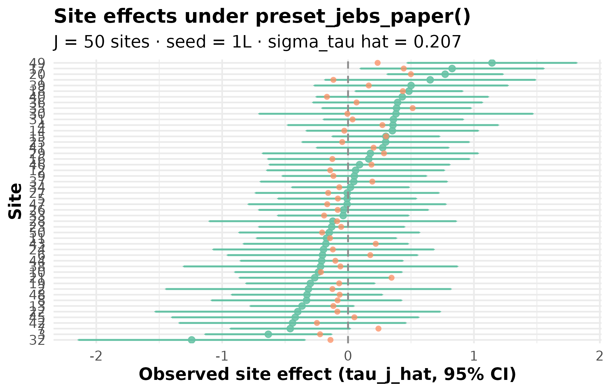
Caterpillar plot of 50 simulated site effects from preset_jebs_paper, ordered left-to-right by absolute estimate, with 95 percent intervals around each observed estimate.

Caterpillar plot. Black points are observed estimates with 95 percent CI bars; the solid horizontal line marks the grand mean. Sites are sorted by absolute estimate. Vertical spread of the dots is your realized between-site heterogeneity (sigma_tau hat = 0.207); bar-width variation across sites is the sampling-error heterogeneity (R = 7.6) set by site-size variation.

Three things to check on the caterpillar:

Vertical spread of the dots. That is your realized site-level heterogeneity. Confirm it numerically against the sigma_tau line in the diagnostic table.
Bar widths across sites. Wide bars are small sites; narrow bars are large sites. The ratio of widest to narrowest is R = 7.6 — meaningful but not pathological for site-size-driven designs.
Rank order across the x-axis. This is exactly what an empirical Bayes estimator will shrink, and the magnitude of shrinkage tracks how much each site’s bar narrows in your downstream analysis.

plot_funnel(dat, caption = FALSE) +
  ggplot2::labs(
    title    = "Precision vs. effect: funnel view",
    subtitle = "Symmetric scatter confirms target rho_S = 0"
  )

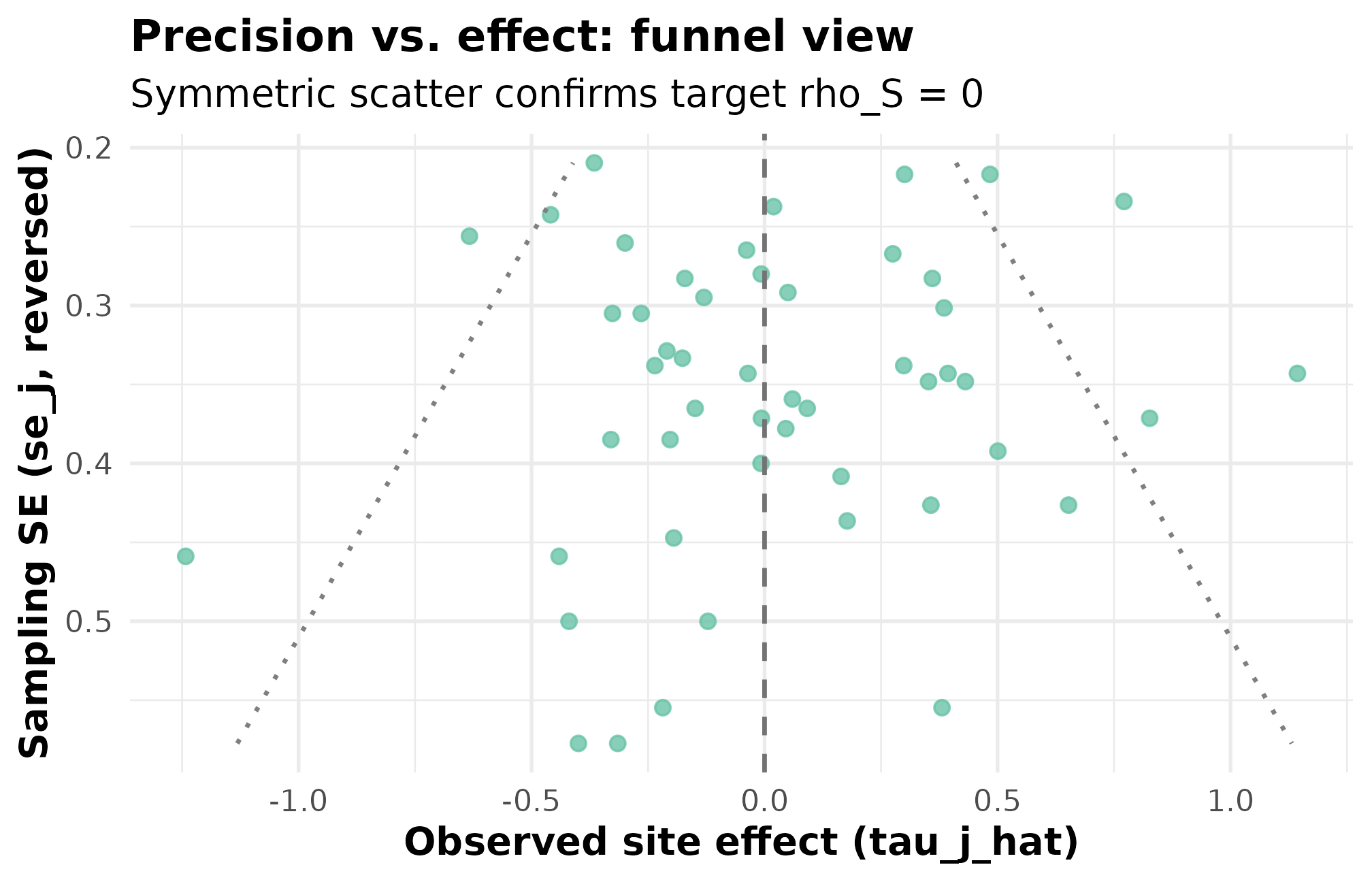
Funnel plot of 50 simulated site effects against their standard errors.

Funnel plot. Standard error on the x-axis (smaller = more precise); observed estimate on the y-axis. Cloud width tapers as SE shrinks, the expected signature when SEs come from site sizes. Roughly symmetric scatter top-to-bottom confirms the rank-correlation target rho_S = 0 (PASS) — small-SE sites are not systematically higher- or lower-effect than large-SE sites.

What to read off the funnel: a biased design would tilt the cloud — small-SE sites would skew toward one side of zero. This funnel is roughly symmetric, the visual signature of the PASS verdict on rank_corr residual. If Maya later modifies the design to induce precision–effect dependence (Layer 3), the cloud will tilt visibly, and the diagnostic flag will flip.

8. Adapt for downstream analysis

Three adapter functions hand the simulation off to specific downstream packages without renaming columns by hand: as_metafor(), as_baggr(), and as_multisitepower().

mf <- as_metafor(dat)
head(mf, 4)
#> # A tibble: 4 × 3
#>       yi     vi   sei
#>    <dbl>  <dbl> <dbl>
#> 1  0.652 0.182  0.426
#> 2 -0.315 0.333  0.577
#> 3 -0.633 0.0656 0.256
#> 4  0.357 0.182  0.426

After as_metafor() the columns are yi (effect estimate), vi (sampling variance), and sei (sampling SE) — the convention metafor::rma() expects. Sibling adapters return the column conventions of the baggr and multisitepower packages. The recipe gallery at Cookbook walks each adapter end-to-end with a fitted model; Adapters and downstream packages gives the formal rename contract.

9. Provenance

A defensible simulation needs a one-line fingerprint Maya can paste into the methods appendix. provenance_string() returns it.

provenance_string(dat)
#> [1] "multisiteDGP 0.1.1 | paradigm=site_size | seed=1 | canonical_hash=b29561b47a40332d | design_hash=cddffb66364a11ee | hash_algo=xxhash64 | R=4.6.0 | hooks=none"

The string carries the package version, the paradigm, the seed, the canonical hash of the simulation output, the design hash, the hash algorithm, the R version, and any active hooks. The canonical hash itself can be pulled directly:

canonical_hash(dat)
#> [1] "b29561b47a40332d"

If a coauthor reruns sim_multisite(preset_jebs_paper(), seed = 1L) on the same package version, that 16-character hash is the contract: identical hash means byte-identical simulation. A different hash flags a drift in the design, the seed, or the package — exactly what a methods reviewer wants to be sure cannot happen silently. You can verify this directly:

dat_repeat <- sim_multisite(design, seed = 1L)
identical(canonical_hash(dat), canonical_hash(dat_repeat))
#> [1] TRUE

See Reproducibility and provenance for how to wire the hash and provenance string into automated audit trails.

10. Where to next

Choosing a preset — the nine built-in presets and when each fits your design.
Diagnostics in practice — the four diagnostic groups (A: scale, B: dependence, C: G-shape fit, D: feasibility) and the plots that go with each.
Calibrating to real data — when you have observed point estimates and SEs you want the simulator to match.
sim_multisite() — full argument reference, including how to override preset fields.
preset_jebs_paper() — the preset used here.

For the methodological foundations — the formal two-stage DGP, the G-distribution catalog, the site-size-driven and direct-precision paths — start with The two-stage DGP and proceed through M2 / M3 / M4 in order.

References

The multisiteDGP data-generating process and the JEBS preset implement the design in Lee et al. (2025). Empirical-Bayes context for site-effect estimation is collected in Walters (2024); applied calibration benchmarks for the education presets are taken from Weiss et al. (2017).

Acknowledgments

This research was supported by the Institute of Education Sciences, U.S. Department of Education, through Grant R305D240078 to the University of Alabama. The opinions expressed are those of the authors and do not represent views of the Institute or the U.S. Department of Education.

Session info

#> R version 4.6.0 (2026-04-24)
#> Platform: x86_64-pc-linux-gnu
#> Running under: Ubuntu 24.04.4 LTS
#> 
#> Matrix products: default
#> BLAS:   /usr/lib/x86_64-linux-gnu/openblas-pthread/libblas.so.3 
#> LAPACK: /usr/lib/x86_64-linux-gnu/openblas-pthread/libopenblasp-r0.3.26.so;  LAPACK version 3.12.0
#> 
#> locale:
#>  [1] LC_CTYPE=C.UTF-8       LC_NUMERIC=C           LC_TIME=C.UTF-8       
#>  [4] LC_COLLATE=C.UTF-8     LC_MONETARY=C.UTF-8    LC_MESSAGES=C.UTF-8   
#>  [7] LC_PAPER=C.UTF-8       LC_NAME=C              LC_ADDRESS=C          
#> [10] LC_TELEPHONE=C         LC_MEASUREMENT=C.UTF-8 LC_IDENTIFICATION=C   
#> 
#> time zone: UTC
#> tzcode source: system (glibc)
#> 
#> attached base packages:
#> [1] stats     graphics  grDevices utils     datasets  methods   base     
#> 
#> other attached packages:
#> [1] ggplot2_4.0.3      multisiteDGP_0.1.1
#> 
#> loaded via a namespace (and not attached):
#>  [1] Matrix_1.7-5        gtable_0.3.6        jsonlite_2.0.0     
#>  [4] dplyr_1.2.1         compiler_4.6.0      tidyselect_1.2.1   
#>  [7] metafor_5.0-1       jquerylib_0.1.4     systemfonts_1.3.2  
#> [10] scales_1.4.0        textshaping_1.0.5   yaml_2.3.12        
#> [13] fastmap_1.2.0       lattice_0.22-9      R6_2.6.1           
#> [16] labeling_0.4.3      generics_0.1.4      knitr_1.51         
#> [19] tibble_3.3.1        desc_1.4.3          bslib_0.10.0       
#> [22] pillar_1.11.1       RColorBrewer_1.1-3  rlang_1.2.0        
#> [25] cachem_1.1.0        mathjaxr_2.0-0      xfun_0.57          
#> [28] fs_2.1.0            sass_0.4.10         S7_0.2.2           
#> [31] cli_3.6.6           pkgdown_2.2.0       withr_3.0.2        
#> [34] magrittr_2.0.5      digest_0.6.39       grid_4.6.0         
#> [37] metadat_1.6-0       nlme_3.1-169        lifecycle_1.0.5    
#> [40] vctrs_0.7.3         evaluate_1.0.5      glue_1.8.1         
#> [43] numDeriv_2016.8-1.1 farver_2.1.2        ragg_1.5.2         
#> [46] rmarkdown_2.31      tools_4.6.0         pkgconfig_2.0.3    
#> [49] htmltools_0.5.9

Lee, J., Che, J., Rabe-Hesketh, S., Feller, A., & Miratrix, L. (2025). Improving the estimation of site-specific effects and their distribution in multisite trials. Journal of Educational and Behavioral Statistics, 50(5), 731–764. https://doi.org/10.3102/10769986241254286

Walters, C. (2024). Empirical bayes methods in labor economics. In Handbook of labor economics (Vol. 5, pp. 183–260). Elsevier. https://doi.org/10.1016/bs.heslab.2024.11.001

Weiss, M. J., Bloom, H. S., Verbitsky-Savitz, N., Gupta, H., Vigil, A. E., & Cullinan, D. N. (2017). How much do the effects of education and training programs vary across sites? Evidence from past multisite randomized trials. Journal of Research on Educational Effectiveness, 10(4), 843–876. https://doi.org/10.1080/19345747.2017.1300719

A1 · Getting started — your first multisite simulation

JoonHo Lee

2026-05-10