M4 · Precision dependence — three injection methods
JoonHo Lee
2026-05-10
Source:vignettes/m4-precision-dependence-theory.Rmd
m4-precision-dependence-theory.RmdAbstract
For methodologists building simulations whose generative
process must encode a controlled coupling between site effects and
reported precision, this vignette walks through the three
precision-dependence injection methods multisiteDGP
exposes — align_rank_corr(),
align_copula_corr(), and
align_hybrid_corr() — one section per method. Each
section gives the mathematical form, what the method preserves
exactly, what it distorts, and when to choose it. You leave with
three side-by-side scatterplots at a common target
,
the rationale for the package’s hybrid default, and a decision
rubric for picking among the three.
1. Why independence fails in real multisite trials
The generative skeleton on which multisiteDGP is built
treats the latent site effect
and the reported sampling variance
as independent. That independence is the design’s null
position: under perfect random allocation, no selection, and
uniform implementation fidelity, knowing how precisely a site was
estimated tells you nothing about that site’s true effect. The M1: The two-stage DGP vignette
derives the joint distribution under that null; the M3: Margin and SE models vignette
derives the two precision margins separately. For a wide swath of
pedagogically clean simulation work, that independence is fine.
Reality, however, departs. The blueprint’s chapter on precision dependence (Ch. 7, Precision Dependence) collects three mechanisms by which empirical multisite trials systematically violate the null. Small studies often report systematically larger or smaller effects than large ones — the canonical funnel-asymmetry pattern that motivates publication-bias diagnostics in meta-analysis (Walters, 2024). Selection on observable site characteristics (catchment breadth, treatment fidelity, baseline outcome variance) couples site-level sample size with site-level effect heterogeneity. And adaptive implementation — sites scaling up or down enrolment based on interim signals — can induce coupling between and even when the original allocation was random. When a methodologist wants to ask “is my estimator robust to the kind of dependence I see in the wild?”, the simulation must be able to inject the dependence on purpose, with a controlled target (Lee et al., 2025).
That is what Layer 3 does. Three exported alignment functions —
align_rank_corr(), align_copula_corr(), and
align_hybrid_corr() — permute the precision margin against
the latent effect to produce a target rank correlation between
(the standardized residual effect) and
.
The three differ in how they permute and consequently in
what they preserve exactly, what they distort, and what they
cost in compute. The rest of this vignette walks them through one at a
time.
# A common reference design used throughout this vignette: J = 80
# sites, the package-canonical Gaussian Layer 1, a moderate site-size
# margin (mean 60, CV 0.4), no covariates. We will plug different
# Layer 3 dependence injectors into this fixed input skeleton.
common_args <- list(
  J         = 80L,
  sigma_tau = 0.20,
  nj_mean   = 60,
  cv        = 0.4,
  seed      = 1L
)
target <- 0.40

# Independence baseline — for every primary call that follows, we want
# the reader to see what the un-injected joint distribution looks like.
des_none <- do.call(multisitedgp_design,
                    c(common_args, dependence = "none"))
dat_none <- sim_multisite(des_none)
dat_none
#> # A multisitedgp_data: 80 sites, paradigm = "site_size"
#> # Realized vs intended:
#> #   I: realized=0.347 (no target)
#> #   R: realized=4.200 (no target)
#> #   sigma_tau: target=0.200, realized=0.180, WARN
#> #   rho_S: target=0.000, realized=0.027, PASS
#> #   rho_S_marg: realized=0.027 (no target)
#> #   Feasibility: WARN (n_eff=28.139)
#> # A tibble: 80 × 7
#>   site_index    z_j   tau_j tau_j_hat  se_j  se2_j   n_j
#>        <int>  <dbl>   <dbl>     <dbl> <dbl>  <dbl> <int>
#> 1          1 -0.626 -0.125    -0.0244 0.237 0.0563    71
#> 2          2  0.184  0.0367   -0.0476 0.354 0.125     32
#> 3          3 -0.836 -0.167     0.106  0.258 0.0667    60
#> 4          4  1.60   0.319     0.596  0.312 0.0976    41
#> 5          5  0.330  0.0659   -0.146  0.343 0.118     34
#> 6          6 -0.820 -0.164     0.396  0.254 0.0645    62
#> # ℹ 74 more rows
#> # Use summary(df) for the full diagnostic report.
The independence baseline is what every dependence-injection method
permutes out of. The realized residual Spearman in
dat_none will sit close to zero up to Monte Carlo noise —
the print method’s rho_S line confirms this. From here,
three sections.
2. The rank-permutation method (align_rank_corr)
2.1 Mathematical form
The rank method takes the input pair
and proposes random pair-swaps on the precision column. A swap is
accepted if the post-swap residual Spearman correlation between
and
is closer to the user’s target rank_corr than before;
otherwise rejected. The procedure terminates when the realized Spearman
lands within tol of the target or when
max_iter swaps have been proposed.
Formally, write for the realized site-to-grid permutation of the pre-alignment precision multiset. The rank aligner returns the that minimizes
over the swap-reachable subspace, with the user’s target. Because is by construction a permutation of the pre-alignment precision values, the empirical marginal of is bit-identical to what came in from Layer 2.
2.2 What the method preserves and distorts
Preserves exactly: the empirical marginal of (as a multiset) and trivially the empirical marginal of (which is never moved). No site has its precision value rounded, smoothed, or resampled — only relabeled.
Distorts: the shape of the joint distribution. The rank aligner cares only about the ordering of relative to ; it has no copula structure, no notion of joint smoothness, and no tail-dependence guarantee. For most applied targets in this is irrelevant — the realized scatter looks like a Gaussian-copula scatter to the eye — but at the boundary the rank aligner can produce visibly “step-shaped” plots because the swap-reachable subspace becomes thinner.
Cost in compute: one acceptance test per proposed swap. For and a target of the algorithm typically converges in a handful of swaps from a near-zero baseline.
# align_rank_corr through the multisitedgp_design front door.
des_rank <- multisitedgp_design(
  J         = 80L,
  sigma_tau = 0.20,
  nj_mean   = 60,
  cv        = 0.4,
  dependence = "rank",
  rank_corr  = target,
  seed       = 1L
)
dat_rank <- sim_multisite(des_rank)
dat_rank
#> # A multisitedgp_data: 80 sites, paradigm = "site_size"
#> # Realized vs intended:
#> #   I: realized=0.347 (no target)
#> #   R: realized=4.200 (no target)
#> #   sigma_tau: target=0.200, realized=0.180, WARN
#> #   rho_S: target=0.400, realized=0.401, PASS
#> #   rho_S_marg: realized=0.401 (no target)
#> #   Feasibility: WARN (n_eff=28.139)
#> # A tibble: 80 × 7
#>   site_index    z_j   tau_j tau_j_hat  se_j  se2_j   n_j
#>        <int>  <dbl>   <dbl>     <dbl> <dbl>  <dbl> <int>
#> 1          1 -0.626 -0.125    -0.0244 0.237 0.0563    71
#> 2          2  0.184  0.0367   -0.0476 0.354 0.125     32
#> 3          3 -0.836 -0.167     0.106  0.258 0.0667    60
#> 4          4  1.60   0.319     0.596  0.312 0.0976    41
#> 5          5  0.330  0.0659   -0.146  0.343 0.118     34
#> 6          6 -0.820 -0.164     0.396  0.254 0.0645    62
#> # ℹ 74 more rows
#> # Use summary(df) for the full diagnostic report.
The print method’s rho_S line shows
target=0.400, realized=0.401, PASS. The hill-climb landed
on the target within tolerance after a handful of swaps. The detailed
dependence diagnostics tell the same story:
attr(dat_rank, "diagnostics")$dependence_diagnostics
#> $method
#> [1] "rank"
#>
#> $target_type
#> [1] "residual_spearman"
#>
#> $target
#> [1] 0.4
#>
#> $achieved
#> [1] 0.4013203
#>
#> $residual
#> [1] 0.001320295
#>
#> $converged
#> [1] TRUE
#>
#> $iterations
#> [1] 4
#>
#> $tol
#> [1] 0.02
converged = TRUE, iterations = 4,
residual = 0.00132. For an
-cell
swap budget the algorithm spent four. The realized Spearman is exact
within the user’s tolerance.
# Marginal preservation: the rank method only reorders precision values,
# so the sorted multisets must coincide bit-for-bit with the baseline.
all.equal(sort(dat_rank$se2_j), sort(dat_none$se2_j))
#> [1] TRUE
The sorted precision multiset coincides with the baseline. No precision value was created, smoothed, or rounded.
2.3 When to choose align_rank_corr
Choose the rank method when:
- You want exact preservation of the precision multiset (the values are calibrated targets — from a real trial, for example — and you cannot tolerate even Monte Carlo perturbation).
- The target is moderate (under or so) and the realized correlation must hit the target tightly.
- You want the fastest no-iteration smoke test in scenarios where copula structure is not part of the analysis.
Avoid the rank method when:
- The target sits near . The swap-reachable subspace narrows and the algorithm may stall before converging.
- You need a smooth copula-shaped joint scatter for a downstream density-based diagnostic.
3. The Gaussian-copula method (align_copula_corr)
3.1 Mathematical form
The copula method draws a correlated latent score
for each site from a bivariate Gaussian with target Pearson correlation
pearson_corr and the rank-normalized
on the other axis. It then sorts the empirical
multiset and assigns the values to sites in the order
implies. Concretely, with
and a draw
the aligner pairs the th-order-statistic of with the site whose has the th rank. No iteration; one pass.
The package’s align_copula_corr() calls the target a
latent Gaussian-copula Pearson correlation. The realized
residual Spearman is approximately the user’s pearson_corr
(the two are within Monte Carlo noise at large
for well-behaved marginals) but not exactly.
3.2 What the method preserves and distorts
Preserves exactly: the empirical marginal of as a multiset (the assignment is by rank of the latent score, so the sorted values are unchanged). And the marginal of , never moved.
Distorts: the realized residual Spearman correlation. The aligner targets the latent Pearson correlation between and the rank-normalized ; the implied residual Spearman is approximately but not exactly, because finite- ranks are discrete. At and , the realized residual Spearman lands modestly above target — the residual diagnostic will show roughly a tenth of a correlation point of slack.
Cost in compute: one -vector latent draw and one sort. The copula aligner is the fastest of the three by a wide margin.
# align_copula_corr — note that the target argument is `pearson_corr`,
# not `rank_corr`. The copula targets a latent Gaussian Pearson
# correlation, and the realized residual Spearman follows from the
# arcsine mapping, with finite-J slack.
des_copula <- multisitedgp_design(
  J            = 80L,
  sigma_tau    = 0.20,
  nj_mean      = 60,
  cv           = 0.4,
  dependence   = "copula",
  pearson_corr = target,
  seed         = 1L
)
dat_copula <- sim_multisite(des_copula)
dat_copula
#> # A multisitedgp_data: 80 sites, paradigm = "site_size"
#> # Realized vs intended:
#> #   I: realized=0.347 (no target)
#> #   R: realized=4.200 (no target)
#> #   sigma_tau: target=0.200, realized=0.180, WARN
#> #   rho_S: target=0.000, realized=0.438, FAIL
#> #   rho_S_marg: realized=0.438 (no target)
#> #   Feasibility: WARN (n_eff=28.139)
#> # A tibble: 80 × 7
#>   site_index    z_j   tau_j tau_j_hat  se_j  se2_j   n_j
#>        <int>  <dbl>   <dbl>     <dbl> <dbl>  <dbl> <int>
#> 1          1 -0.626 -0.125    0.0672  0.272 0.0741    54
#> 2          2  0.184  0.0367   0.297   0.252 0.0635    63
#> 3          3 -0.836 -0.167   -0.100   0.298 0.0889    45
#> 4          4  1.60   0.319    0.00342 0.359 0.129     31
#> 5          5  0.330  0.0659   0.348   0.243 0.0588    68
#> 6          6 -0.820 -0.164   -0.894   0.365 0.133     30
#> # ℹ 74 more rows
#> # Use summary(df) for the full diagnostic report.
The print method’s rho_S line shows
target=0.000, realized=0.438, FAIL. Two things to read: (a)
the design’s registered rank-target slot is empty (the user
passed pearson_corr, not rank_corr), so the
diagnostic infrastructure has nothing to compare the realized Spearman
against — that is what target=0.000 means in this row; and
(b) the realized Spearman is
,
modestly above the latent Pearson target of
.
The detailed diagnostics give the full story:
attr(dat_copula, "diagnostics")$dependence_diagnostics
#> $method
#> [1] "copula"
#>
#> $mode
#> [1] "empirical_rank_pairing"
#>
#> $preservation
#> [1] "empirical_multiset"
#>
#> $target_type
#> [1] "latent_gaussian_pearson"
#>
#> $target
#> [1] 0.4
#>
#> $achieved
#> [1] 0.5029913
#>
#> $achieved_latent_pearson
#> [1] 0.5029913
#>
#> $achieved_spearman
#> [1] 0.4383956
#>
#> $residual
#> [1] 0.1029913
#>
#> $ties_method
#> [1] "average"
#>
#> $rng_draws
#> [1] 80
#>
#> $converged
#> [1] NA
#>
#> $iterations
#> [1] 0
#>
#> $tol
#> [1] NA
The aligner reports target = 0.40 (interpreted as latent
Gaussian Pearson), achieved = 0.503 on the latent Pearson
scale, and achieved_spearman = 0.438 on the residual
Spearman scale. The residual = 0.103 is the slack on the
latent Pearson; the
finite-
Spearman slack is smaller. mode = "empirical_rank_pairing"
documents the assignment rule;
preservation = "empirical_multiset" confirms that the
precision margin is unchanged.
Bit-identical sorted multisets, again. The copula method preserves the precision values as exactly as the rank method does — the empirical-rank pairing variant of the copula aligner uses ordering to assign, never resampling.
3.3 When to choose align_copula_corr
Choose the copula method when:
- The simulation lives on the direct-precision path (Paradigm B in the blueprint) and the natural target is a latent Gaussian-copula correlation rather than a realized rank correlation.
- You need the fastest method (no iteration) and can tolerate finite- slack on the realized residual Spearman.
- Downstream diagnostics consume the Gaussian-copula joint shape itself (density-overlay plots, copula-density estimators).
Avoid the copula method when:
- The realized residual Spearman must hit the target tightly. Use hybrid (the next section) instead.
- You want to specify the target as a Spearman directly. The copula takes a latent Pearson; the back-mapping gets you part of the way, but the finite- slack is on the realized side.
4. The hybrid method (align_hybrid_corr)
4.1 Mathematical form
The hybrid method runs the copula aligner first as an initialization
pass, then runs the rank aligner on the result as a polishing pass. The
copula stage lands the realized scatter in the right neighborhood of the
joint distribution — Gaussian-copula-shaped, smooth, marginals
preserved. The rank stage spends a handful of swaps cleaning up the
finite-
slack on the realized residual Spearman, driving it to within
tol of rank_corr.
The composition keeps the copula stage’s Gaussian-copula shape
(modulo a small polishing perturbation) and inherits the rank stage’s
tight target accuracy. The init and polish
arguments expose the two-stage structure: init = "copula"
(default) gives the copula initialization;
polish = "hill_climb" (default) gives the rank polish.
Either stage can be replaced or skipped.
4.2 What the method preserves and distorts
Preserves exactly: the empirical marginal of . Both stages assign by rank, so the sorted precision multiset is unchanged.
Preserves approximately: the Gaussian-copula joint shape. The polishing pass perturbs the copula scatter slightly — far less than a pure rank aligner from a cold start, because most swaps are not needed.
Distorts: essentially nothing of practical concern
at typical applied targets. At
and
,
the realized residual Spearman lands within tol = 0.02 of
the target, the precision multiset is bit-identical, and the joint
scatter retains the copula stage’s smooth shape.
Cost in compute: the copula stage’s -vector latent draw plus the rank stage’s polishing swaps. For typical applied targets the polishing budget is negligible. At boundary targets () the polishing burden grows but stays under the pure-rank cost, because the copula initialization placed the scatter in the right neighborhood.
# align_hybrid_corr is the package default. The dependence_spec slot
# of the design carries `dependence = "hybrid"` automatically when the
# user passes `rank_corr` without specifying a method, but here we
# pass it explicitly for clarity.
des_hybrid <- multisitedgp_design(
  J          = 80L,
  sigma_tau  = 0.20,
  nj_mean    = 60,
  cv         = 0.4,
  dependence = "hybrid",
  rank_corr  = target,
  seed       = 1L
)
dat_hybrid <- sim_multisite(des_hybrid)
dat_hybrid
#> # A multisitedgp_data: 80 sites, paradigm = "site_size"
#> # Realized vs intended:
#> #   I: realized=0.347 (no target)
#> #   R: realized=4.200 (no target)
#> #   sigma_tau: target=0.200, realized=0.180, WARN
#> #   rho_S: target=0.400, realized=0.400, PASS
#> #   rho_S_marg: realized=0.400 (no target)
#> #   Feasibility: WARN (n_eff=28.139)
#> # A tibble: 80 × 7
#>   site_index    z_j   tau_j tau_j_hat  se_j  se2_j   n_j
#>        <int>  <dbl>   <dbl>     <dbl> <dbl>  <dbl> <int>
#> 1          1 -0.626 -0.125    0.0672  0.272 0.0741    54
#> 2          2  0.184  0.0367   0.297   0.252 0.0635    63
#> 3          3 -0.836 -0.167   -0.100   0.298 0.0889    45
#> 4          4  1.60   0.319    0.00342 0.359 0.129     31
#> 5          5  0.330  0.0659   0.348   0.243 0.0588    68
#> 6          6 -0.820 -0.164   -0.894   0.365 0.133     30
#> # ℹ 74 more rows
#> # Use summary(df) for the full diagnostic report.
The print method’s rho_S line shows
target=0.400, realized=0.400, PASS. The hybrid landed
exactly on target. The detailed diagnostics expose the two-stage
internal structure:
attr(dat_hybrid, "diagnostics")$dependence_diagnostics
#> $method
#> [1] "hybrid"
#>
#> $mode
#> [1] "empirical_rank_pairing"
#>
#> $preservation
#> [1] "empirical_multiset"
#>
#> $target_type
#> [1] "residual_spearman"
#>
#> $target
#> [1] 0.4
#>
#> $pearson_init
#> [1] 0.4158234
#>
#> $achieved
#> [1] 0.4000305
#>
#> $achieved_spearman
#> [1] 0.4000305
#>
#> $residual
#> [1] 3.051745e-05
#>
#> $converged
#> [1] TRUE
#>
#> $iterations
#> [1] 1
#>
#> $tol
#> [1] 0.02
#>
#> $ties_method
#> [1] "average"
#>
#> $init
#> [1] "copula"
#>
#> $polish
#> [1] "hill_climb"
#>
#> $rng_draws
#> [1] 80
#>
#> $init_diagnostics
#> $init_diagnostics$method
#> [1] "copula"
#>
#> $init_diagnostics$mode
#> [1] "empirical_rank_pairing"
#>
#> $init_diagnostics$preservation
#> [1] "empirical_multiset"
#>
#> $init_diagnostics$target_type
#> [1] "latent_gaussian_pearson"
#>
#> $init_diagnostics$target
#> [1] 0.4158234
#>
#> $init_diagnostics$achieved
#> [1] 0.5156992
#>
#> $init_diagnostics$achieved_latent_pearson
#> [1] 0.5156992
#>
#> $init_diagnostics$achieved_spearman
#> [1] 0.4466501
#>
#> $init_diagnostics$residual
#> [1] 0.09987583
#>
#> $init_diagnostics$ties_method
#> [1] "average"
#>
#> $init_diagnostics$rng_draws
#> [1] 80
#>
#> $init_diagnostics$converged
#> [1] NA
#>
#> $init_diagnostics$iterations
#> [1] 0
#>
#> $init_diagnostics$tol
#> [1] NA
#>
#>
#> $polish_diagnostics
#> $polish_diagnostics$method
#> [1] "rank"
#>
#> $polish_diagnostics$target_type
#> [1] "residual_spearman"
#>
#> $polish_diagnostics$target
#> [1] 0.4
#>
#> $polish_diagnostics$achieved
#> [1] 0.4000305
#>
#> $polish_diagnostics$residual
#> [1] 3.051745e-05
#>
#> $polish_diagnostics$converged
#> [1] TRUE
#>
#> $polish_diagnostics$iterations
#> [1] 1
#>
#> $polish_diagnostics$tol
#> [1] 0.02
The list is structured as init (the copula stage’s
diagnostics) and polish (the rank stage’s). The init stage
reports the copula target it received from the front door (the rank
target was mapped to its latent-Pearson cousin by the design
constructor) and the realized Spearman it landed on after one pass. The
polish stage took iterations = 1 to drive the realized
Spearman to 0.4000305, landing with
residual = 3.05e-05. Notice how few swaps polishing needed
— copula initialization did the heavy lifting.
Bit-identical sorted multisets. The hybrid preserves the precision margin as exactly as either pure method does.
4.3 When to choose align_hybrid_corr
Choose the hybrid method when:
- You want both tight realized-Spearman accuracy and a Gaussian-copula-shaped joint scatter.
- The simulation will be cited or audited (the hybrid is the package default; reaching for it is the “no surprise” choice).
- The target sits in the typical applied range () where the copula initialization places the scatter close to target and the polishing budget is small.
Avoid the hybrid method when:
- You need raw speed and can tolerate the copula-only slack — use
align_copula_corr()directly. - The simulation specifically demands no Monte Carlo noise on the
joint scatter (e.g., a deterministic-replay smoke test) — use
align_rank_corr()from a cold start, which uses nornorm()draws.
5. Side-by-side scatter comparison
The three methods all target the same realized residual correlation — roughly — but the shape of the joint scatter is where they differ. Building three plots on the same axes shows what each method emphasizes.
# Stack the three datasets with a method label for ggplot's facet grid.
to_scatter <- function(dat, label) {
  data.frame(
    method = label,
    z_j    = dat$z_j,
    se2_j  = dat$se2_j
  )
}

scatter_df <- rbind(
  to_scatter(dat_rank,   "rank"),
  to_scatter(dat_copula, "copula"),
  to_scatter(dat_hybrid, "hybrid")
)
scatter_df$method <- factor(
  scatter_df$method,
  levels = c("rank", "copula", "hybrid")
)
head(scatter_df)
#>   method        z_j      se2_j
#> 1   rank -0.6264538 0.05633803
#> 2   rank  0.1836433 0.12500000
#> 3   rank -0.8356286 0.06666667
#> 4   rank  1.5952808 0.09756098
#> 5   rank  0.3295078 0.11764706
#> 6   rank -0.8204684 0.06451613
ggplot(subset(scatter_df, method == "rank"),
       aes(x = z_j, y = se2_j)) +
  geom_point(alpha = 0.7, color = "steelblue", size = 2) +
  geom_smooth(method = "loess", se = FALSE,
              color = "darkblue", linewidth = 0.7) +
  labs(
    title = "Rank-permutation method (rank_corr = 0.40)",
    x = expression(z[j]~"(standardized residual effect)"),
    y = expression(widehat(se)[j]^2~"(sampling variance)")
  ) +
  theme_minimal(base_size = 11)
Rank-method scatter at target . Higher pairs with higher across the full range, and the precision values along the y-axis match the baseline multiset bit-for-bit, confirming the realized residual Spearman lands within tolerance of 0.40 by reordering — not resampling.
ggplot(subset(scatter_df, method == "copula"),
       aes(x = z_j, y = se2_j)) +
  geom_point(alpha = 0.7, color = "darkorange", size = 2) +
  geom_smooth(method = "loess", se = FALSE,
              color = "darkred", linewidth = 0.7) +
  labs(
    title = "Gaussian-copula method (pearson_corr = 0.40)",
    x = expression(z[j]~"(standardized residual effect)"),
    y = expression(widehat(se)[j]^2~"(sampling variance)")
  ) +
  theme_minimal(base_size = 11)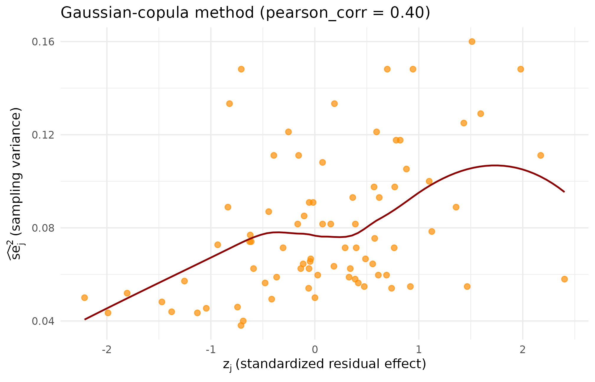
Copula-method scatter at the same target. The Gaussian-copula structure produces a smoother, more elliptical cloud than the rank scatter; the realized residual Spearman lands modestly above target (), confirming the finite- slack flagged in the dependence diagnostics.
ggplot(subset(scatter_df, method == "hybrid"),
       aes(x = z_j, y = se2_j)) +
  geom_point(alpha = 0.7, color = "darkgreen", size = 2) +
  geom_smooth(method = "loess", se = FALSE,
              color = "darkgreen", linewidth = 0.7) +
  labs(
    title = "Hybrid method (rank_corr = 0.40)",
    x = expression(z[j]~"(standardized residual effect)"),
    y = expression(widehat(se)[j]^2~"(sampling variance)")
  ) +
  theme_minimal(base_size = 11)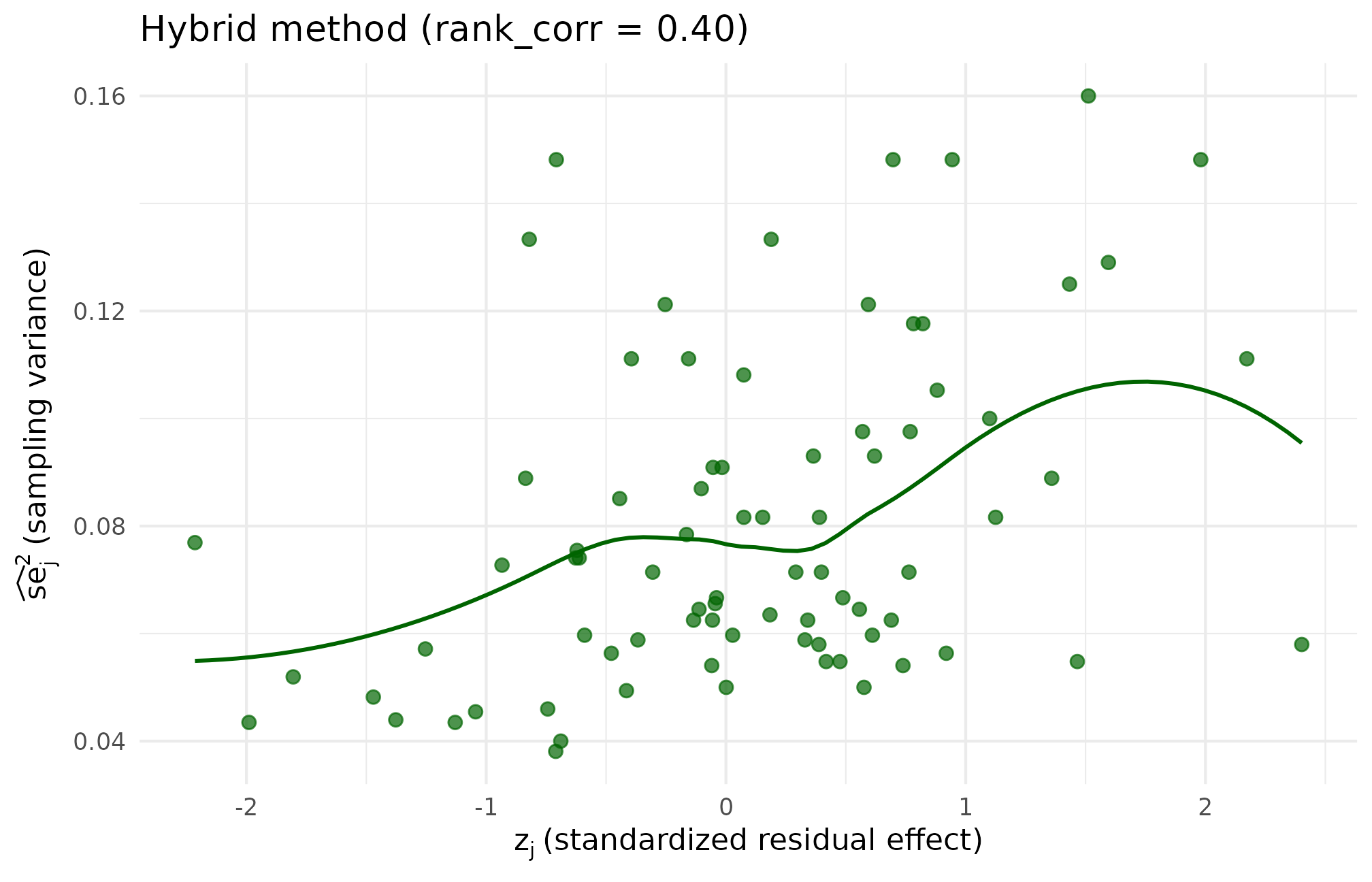
Hybrid-method scatter at the same target. The cloud retains the copula method’s smooth elliptical shape but the realized residual Spearman lands within 0.0001 of 0.40 after a single polishing swap, confirming the recommended default delivers both joint-shape smoothness and target accuracy.
The three plots tell a consistent story. The rank method’s scatter shows the same underlying pairs, just permuted. The copula method’s scatter looks smoother because the assignment was driven by a continuous latent-score draw rather than by individual swap moves. The hybrid method’s scatter inherits the copula stage’s smoothness and the rank stage’s target accuracy, which is why it is the package default.
To make the exact match of marginals across methods concrete, sorting the precision column from each dataset gives the same sequence by construction:
# Same multiset, different assignment.
identical(
  list(sort(dat_rank$se2_j), sort(dat_copula$se2_j),
       sort(dat_hybrid$se2_j), sort(dat_none$se2_j)),
  rep(list(sort(dat_none$se2_j)), 4)
)
#> [1] TRUE
Four sorted vectors, all identical. The methods differ only in which site receives which precision value.
6. Recommended default and decision rubric
The package’s recommended default is hybrid. For production designs, the hybrid combines:
- The copula initialization’s smooth Gaussian-copula joint shape (the scatter looks like what most readers expect of a “correlated and ” sample).
- The rank polishing pass’s tight target accuracy (the realized
residual Spearman lands within
tol = 0.02of target). - Bit-exact preservation of the pre-alignment precision multiset.
The cost is modest: one -vector latent Gaussian draw plus a small number of polishing swaps. For typical applied targets (the bulk of applied multisite-trial work, and certainly the JEBS-reproduction band studied in Lee et al. (2025)), the polishing budget is negligible — at and target , polishing took a single iteration.
The other two methods are not deprecated; they have specific niches:
-
align_rank_corr()is the right pick for fast smoke tests where the joint shape is irrelevant and only the realized Spearman matters, or for deterministic-replay scenarios where nornorm()draws are desired. -
align_copula_corr()is the right pick for direct-precision designs in meta-analysis settings where the natural target is a latent Pearson correlation and the finite- slack on the realized Spearman is acceptable.
A compact decision rule:
| Need | Method | Rationale |
|---|---|---|
| Production / cited simulation | align_hybrid_corr() |
Default; smooth shape + tight target accuracy |
| Fast smoke test, joint shape irrelevant | align_rank_corr() |
Fewest swaps; no rnorm() draws; exact multiset |
| Direct-precision designs | align_copula_corr() |
Latent-Pearson target is natural; one-pass speed |
| Bit-deterministic replay | align_rank_corr() |
Hill-climb proposes via sample.int(); copula uses
rnorm()
|
| Boundary targets () | align_hybrid_corr() |
Copula init narrows the search; pure rank may stall |
For users who pass arguments to multisitedgp_design()
without specifying dependence explicitly, the constructor
selects the appropriate method based on which target argument is
supplied. Passing rank_corr without dependence
triggers an error so the user must opt in to a method by name.
7. A note on what is not modelled
All three methods produce joint scatters with zero asymptotic upper tail dependence:
$$ \lambda_U \;=\; \lim_{u \to 1^-} \Pr\!\bigl(F_{\widehat{se}^{\,2}}(\widehat{se}_j^{\,2}) > u \;\bigm|\; F_{\tau}(\tau_j) > u\bigr) \;=\; 0. $$
Real-world mechanisms that one might suspect of inducing tail-coupling (rare-population sites with simultaneously large effects and large sampling variance) are not represented by any of the three methods. A Student- copula extension is on the medium-term roadmap (the blueprint Ch. 7 §4 Tail Dependence Caveat flags this as a future item). For JEBS-band simulations the body-of-distribution dependence captured by the three current methods is sufficient — the empirical-Bayes estimators studied in Lee et al. (2025) are most sensitive to the body, not the tails.
8. Where to next
- A4: Covariates and precision dependence shows the three methods composing with the covariate machinery — what changes when is the covariate-residualized standardized effect rather than the raw effect.
-
A6: Case study — multisite
trial walks through a full applied workflow that uses
align_hybrid_corr()as the default Layer 3 injector and shows the downstream diagnostics that read off the dependence target. - M3: Margin and SE models derives the two precision margins on which Layer 3 acts — site-size-driven and direct-precision — and shows the cross-paradigm guards.
-
M7: Reproducibility and
provenance covers the seed-and-hash discipline that makes hybrid
simulations bit-replayable across users and machines despite the copula
stage’s
rnorm()draws.
The reference pages give the full argument lists and contracts: align_rank_corr(),
align_copula_corr(),
align_hybrid_corr(),
and the front-door wrapper multisitedgp_design().
Acknowledgments
This research was supported by the Institute of Education Sciences, U.S. Department of Education, through Grant R305D240078 to the University of Alabama. The opinions expressed are those of the authors and do not represent views of the Institute or the U.S. Department of Education.
Session info
#> R version 4.6.0 (2026-04-24)
#> Platform: x86_64-pc-linux-gnu
#> Running under: Ubuntu 24.04.4 LTS
#>
#> Matrix products: default
#> BLAS:   /usr/lib/x86_64-linux-gnu/openblas-pthread/libblas.so.3
#> LAPACK: /usr/lib/x86_64-linux-gnu/openblas-pthread/libopenblasp-r0.3.26.so;  LAPACK version 3.12.0
#>
#> locale:
#>  [1] LC_CTYPE=C.UTF-8       LC_NUMERIC=C           LC_TIME=C.UTF-8
#>  [4] LC_COLLATE=C.UTF-8     LC_MONETARY=C.UTF-8    LC_MESSAGES=C.UTF-8
#>  [7] LC_PAPER=C.UTF-8       LC_NAME=C              LC_ADDRESS=C
#> [10] LC_TELEPHONE=C         LC_MEASUREMENT=C.UTF-8 LC_IDENTIFICATION=C
#>
#> time zone: UTC
#> tzcode source: system (glibc)
#>
#> attached base packages:
#> [1] stats     graphics  grDevices utils     datasets  methods   base
#>
#> other attached packages:
#> [1] ggplot2_4.0.3      multisiteDGP_0.1.1
#>
#> loaded via a namespace (and not attached):
#>  [1] Matrix_1.7-5       gtable_0.3.6       jsonlite_2.0.0     dplyr_1.2.1
#>  [5] compiler_4.6.0     tidyselect_1.2.1   nleqslv_3.3.7      jquerylib_0.1.4
#>  [9] splines_4.6.0      systemfonts_1.3.2  scales_1.4.0       textshaping_1.0.5
#> [13] yaml_2.3.12        fastmap_1.2.0      lattice_0.22-9     R6_2.6.1
#> [17] labeling_0.4.3     generics_0.1.4     knitr_1.51         tibble_3.3.1
#> [21] desc_1.4.3         bslib_0.10.0       pillar_1.11.1      RColorBrewer_1.1-3
#> [25] rlang_1.2.0        cachem_1.1.0       xfun_0.57          fs_2.1.0
#> [29] sass_0.4.10        S7_0.2.2           cli_3.6.6          mgcv_1.9-4
#> [33] pkgdown_2.2.0      withr_3.0.2        magrittr_2.0.5     digest_0.6.39
#> [37] grid_4.6.0         nlme_3.1-169       lifecycle_1.0.5    vctrs_0.7.3
#> [41] evaluate_1.0.5     glue_1.8.1         farver_2.1.2       ragg_1.5.2
#> [45] rmarkdown_2.31     tools_4.6.0        pkgconfig_2.0.3    htmltools_0.5.9