M7 · Reproducibility and provenance • multisiteDGP

Abstract

For applied researchers who have already run a simulation and now want to make sure the result is reproducible — by them tomorrow, by a coauthor next month, by a reviewer next year. This vignette walks through the five-step workflow multisiteDGP is designed around: set the seed, capture the provenance string, capture the canonical hash, save a manifest, and verify the hash on rerun. You leave with a one-line provenance fingerprint, a 16-character hash, a saved manifest tibble, and a clear sense of what the package guarantees and where the contract can break.

1. Why reproducibility matters

You ran a simulation. The numbers in your draft — the realized between-site standard deviation, the shrinkage benefit, the funnel plot — all came from a single call to sim_multisite() on a single afternoon. Six months from now, a reviewer asks whether you can reproduce the results, or a coauthor wants to extend them, or a graduate student tries to swap in a new preset and discovers the output looks different from the one in your appendix. At that point you need to be able to say, with one line of evidence: the simulation that produced Figure 3 is byte-identical to this rerun, or, equivalently, the contract is broken — here is exactly which ingredient changed. That one-line evidence is what canonical_hash() and provenance_string() give you, and what the rest of this vignette walks through.

2. The four-piece kit

multisiteDGP ships four pieces of machinery for the job. Two are exported functions you call directly; one is a policy the package enforces internally on your behalf; one is a pattern (the “manifest”) you assemble per project.

canonical_hash(x) — the 16-character xxhash64 content fingerprint of a simulation object, a design object, or any data-frame-shaped result. It normalizes column order, drops row names, restricts to a stable diagnostics allowlist, and replaces callback functions with presence sentinels. Two runs with the same package version, seed, and design produce the same hash; any meaningful drift produces a different hash.
provenance_string(x) — a single pipe-delimited line carrying package version, paradigm, seed, canonical hash, design hash, hash algorithm, R version, and any active hooks. Drop it in the methods appendix or a figure caption; it is the smallest unit a reviewer needs to identify the run.
The local-seed-stream policy — internally the package never manufactures seeds from the caller’s global RNG state. Whenever sim_multisite() or sim_meta() needs to allocate per-row seeds (for example, when running a design_grid()), it does so with withr::with_seed() inside an isolated stream so your ambient set.seed() is never disturbed. The practical consequence is that running unrelated code between two sim_multisite() calls with the same seed = 1L cannot change either result.
The golden-fixture manifest — a tibble (or row in a registry) recording the artifact name, package version, preset, seed, canonical hash, design hash, hash algorithm, R version, and platform for one specific simulation. Saving this alongside a paper draft, or committing it to your project repo, is what turns the hash from a computation into a contract.

The first two are the user-facing surface. The third is invisible. The fourth is yours to assemble. Sections 3 through 5 below walk through how the four pieces fit together in a five-step workflow.

3. Workflow walkthrough — pinning a single artifact

The walkthrough is structured around one running example: you have just run a simulation with preset_jebs_paper() at seed = 1L, and you want to pin it. The example is the same one used as the package’s smoke check, so the canonical hash you will see — c52e75f276d82836 — is also documented in the vignettes/_vignette-frontmatter-template.txt file as the package-level determinism check. If your local rerun produces this exact hash, the version of the package you have installed is in sync with the published reference.

3.1 Step 1 — set the seed

The seed is the entry point to determinism. The package follows the convention used by lee2025improving and the JEBS preset: pass an integer to the seed argument of every primary call, do not rely on the ambient global RNG state. The setup chunk also calls set.seed(1L) for any helper code outside the primary calls.

set.seed(1L)

A common pitfall: setting the global seed but forgetting to pass seed = 1L to sim_multisite(). The two are not interchangeable. The argument carries the seed through the local seed stream the package allocates internally; the global call only protects helpers that draw from runif() directly.

3.2 Step 2 — run the simulation and capture `provenance_string()`

Run the simulation. The result is a multisitedgp_data object — a tibble with simulation-specific attributes for design, paradigm, diagnostics, and provenance.

dat <- sim_multisite(preset_jebs_paper(), seed = 1L)
dat
#> # A multisitedgp_data: 50 sites, paradigm = "site_size"
#> # Realized vs intended:
#> #   I: realized=0.250 (no target)
#> #   R: realized=7.583 (no target)
#> #   sigma_tau: target=0.200, realized=0.207, PASS
#> #   rho_S: target=0.000, realized=-0.193, PASS
#> #   rho_S_marg: realized=-0.193 (no target)
#> #   Feasibility: WARN (n_eff=13.098)
#> # A tibble: 50 × 7
#>   site_index    z_j   tau_j tau_j_hat  se_j  se2_j   n_j
#>        <int>  <dbl>   <dbl>     <dbl> <dbl>  <dbl> <int>
#> 1          1 -0.582 -0.116    0.652   0.426 0.182     22
#> 2          2 -0.619 -0.124   -0.315   0.577 0.333     12
#> 3          3 -1.11  -0.222   -0.633   0.256 0.0656    61
#> 4          4  1.36   0.273    0.357   0.426 0.182     22
#> 5          5 -0.405 -0.0809  -0.00723 0.280 0.0784    51
#> 6          6  0.884  0.177   -0.203   0.385 0.148     27
#> # ℹ 44 more rows
#> # Use summary(df) for the full diagnostic report.

Now ask the object for its one-line provenance fingerprint.

provenance_string(dat)
#> [1] "multisiteDGP 0.1.1 | paradigm=site_size | seed=1 | canonical_hash=b29561b47a40332d | design_hash=cddffb66364a11ee | hash_algo=xxhash64 | R=4.6.0 | hooks=none"

Read the line left to right: package version, paradigm (the site-size-driven path of lee2025improving, versus the direct-precision path used in A7), seed, content hash of the realized data, fingerprint of the design alone, hash algorithm, R version, and active callbacks (none because preset_jebs_paper() registers no user-supplied g_fn, se_fn, or dependence callback). This is the line you paste into the methods appendix; it is enough for a reviewer to know what was run.

3.3 Step 3 — capture `canonical_hash()` separately

You do not strictly need to capture the hash separately — it appears inside the provenance string. But the hash on its own is the contract you will check programmatically, so it is worth pulling it into a named variable.

h <- canonical_hash(dat)
h
#> [1] "b29561b47a40332d"

Two things are worth noting about what the hash is and is not. It is content-canonical: column order, row names, and the inclusion of non-numeric diagnostics do not affect it. The package sorts columns before hashing and restricts diagnostics to a stable allowlist (I_hat, R_hat, rho_S_residual, rho_S_marginal, rho_P_residual, rho_P_marginal, sigma_tau_resid, sigma_tau_marg). It is callback-presence-sensitive: if a custom g_fn was registered, the hash records that a function was present without hashing the function body or its enclosing environment. Replacing one user callback with another that produces the same output gives a different hash, which is the conservative behavior for an audit trail.

A second hash — the design hash — fingerprints the design object without running the simulation:

design_hash <- canonical_hash(preset_jebs_paper())
design_hash
#> [1] "0f01529be4a49eb4"

This is useful when you want to verify that two collaborators are working from the same design specification before they bother running the simulation. Equal design_hash, equal seed, and equal package version is the three-way agreement that licenses an equality check on canonical_hash(dat).

3.4 Step 4 — save a manifest

The manifest is a one-row tibble (or one row in a per-project registry) that records everything a future rerun would need. There is no built-in save_manifest() function — the manifest is a pattern, not an object — so the snippet below shows the canonical shape. Saving the result as a CSV alongside your paper draft, or committing it to your project repo, is what closes the loop.

manifest <- tibble::tibble(
  artifact       = "fig3_jebs_paper_seed1",
  pkg_version    = as.character(utils::packageVersion("multisiteDGP")),
  preset         = "preset_jebs_paper",
  seed           = 1L,
  paradigm       = attr(dat, "paradigm", exact = TRUE),
  canonical_hash = canonical_hash(dat),
  design_hash    = canonical_hash(preset_jebs_paper()),
  hash_algo      = "xxhash64",
  R_version      = paste(R.version$major, R.version$minor, sep = "."),
  platform       = R.version$platform,
  recorded_at    = format(Sys.time(), "%Y-%m-%dT%H:%M:%S%z")
)
manifest
#> # A tibble: 1 × 11
#>   artifact          pkg_version preset  seed paradigm canonical_hash design_hash
#>   <chr>             <chr>       <chr>  <int> <chr>    <chr>          <chr>      
#> 1 fig3_jebs_paper_… 0.1.1       prese…     1 site_si… b29561b47a403… 0f01529be4…
#> # ℹ 4 more variables: hash_algo <chr>, R_version <chr>, platform <chr>,
#> #   recorded_at <chr>

Pick the artifact slot to match the figure or table the simulation feeds. The pkg_version is the most-watched field — this is the column that, when it changes, is the most common explanation for a hash mismatch on a rerun a year later. The recorded_at timestamp is for forensic ordering only; it is not part of the determinism contract.

In production work the manifest is typically saved as outputs/manifests/<artifact>.csv and the bare hash as outputs/manifests/<artifact>.hash, both committed to the project repo. A simple convention is enough; nothing in multisiteDGP prescribes a specific layout.

3.5 Step 5 — verify the hash on rerun

You — or your reviewer, or your future self — now want to verify that a rerun of sim_multisite(preset_jebs_paper(), seed = 1L) produces the same simulation. The check is a one-liner.

dat_rerun <- sim_multisite(preset_jebs_paper(), seed = 1L)
identical(canonical_hash(dat_rerun), manifest$canonical_hash)
#> [1] TRUE

TRUE is the contract holding. If the comparison returns FALSE, section 5 below walks through the candidate explanations in order of likelihood (R version, package version, OS).

4. Hash stability under reseed — a visual check

It is worth seeing the hash behavior with your own eyes once. The plot below runs sim_multisite(preset_jebs_paper(), seed = s) for ten values of s, then plots the resulting canonical_hash as a factor. The bar for seed = 1L is repeated five times under deliberately scrambled ambient global RNG state to confirm that the local seed stream insulates the simulation from caller state — the five repeats produce the same hash. The other nine bars are nine different seeds; each gives a different hash.

hash_grid <- function() {
  out <- vector("list", 14L)
  # Five repeats of seed = 1, with global RNG state deliberately scrambled.
  for (k in seq_len(5L)) {
    set.seed(7919L + k * 13L)
    .junk <- runif(100L)
    d <- sim_multisite(preset_jebs_paper(), seed = 1L)
    out[[k]] <- tibble::tibble(
      run = sprintf("rep%02d (seed=1)", k),
      hash = canonical_hash(d),
      seed = 1L
    )
  }
  # Nine more seeds, each once.
  more_seeds <- c(2L, 3L, 4L, 5L, 7L, 11L, 13L, 21L, 42L)
  for (j in seq_along(more_seeds)) {
    s <- more_seeds[[j]]
    d <- sim_multisite(preset_jebs_paper(), seed = s)
    out[[5L + j]] <- tibble::tibble(
      run = sprintf("seed=%d", s),
      hash = canonical_hash(d),
      seed = s
    )
  }
  dplyr::bind_rows(out)
}

hash_tbl <- hash_grid()

ggplot(hash_tbl, ggplot2::aes(x = run, y = 1, fill = hash)) +
  ggplot2::geom_col(width = 0.85) +
  ggplot2::coord_flip() +
  ggplot2::scale_fill_viridis_d(option = "C", guide = "none") +
  ggplot2::labs(
    title = "Canonical hash is stable under reseed and changes with seed",
    subtitle = "preset_jebs_paper() · ambient global state varies across rep01-rep05",
    x = NULL, y = NULL
  ) +
  ggplot2::theme_minimal(base_size = 11) +
  ggplot2::theme(
    axis.text.x = ggplot2::element_blank(),
    axis.ticks.x = ggplot2::element_blank(),
    panel.grid = ggplot2::element_blank()
  )

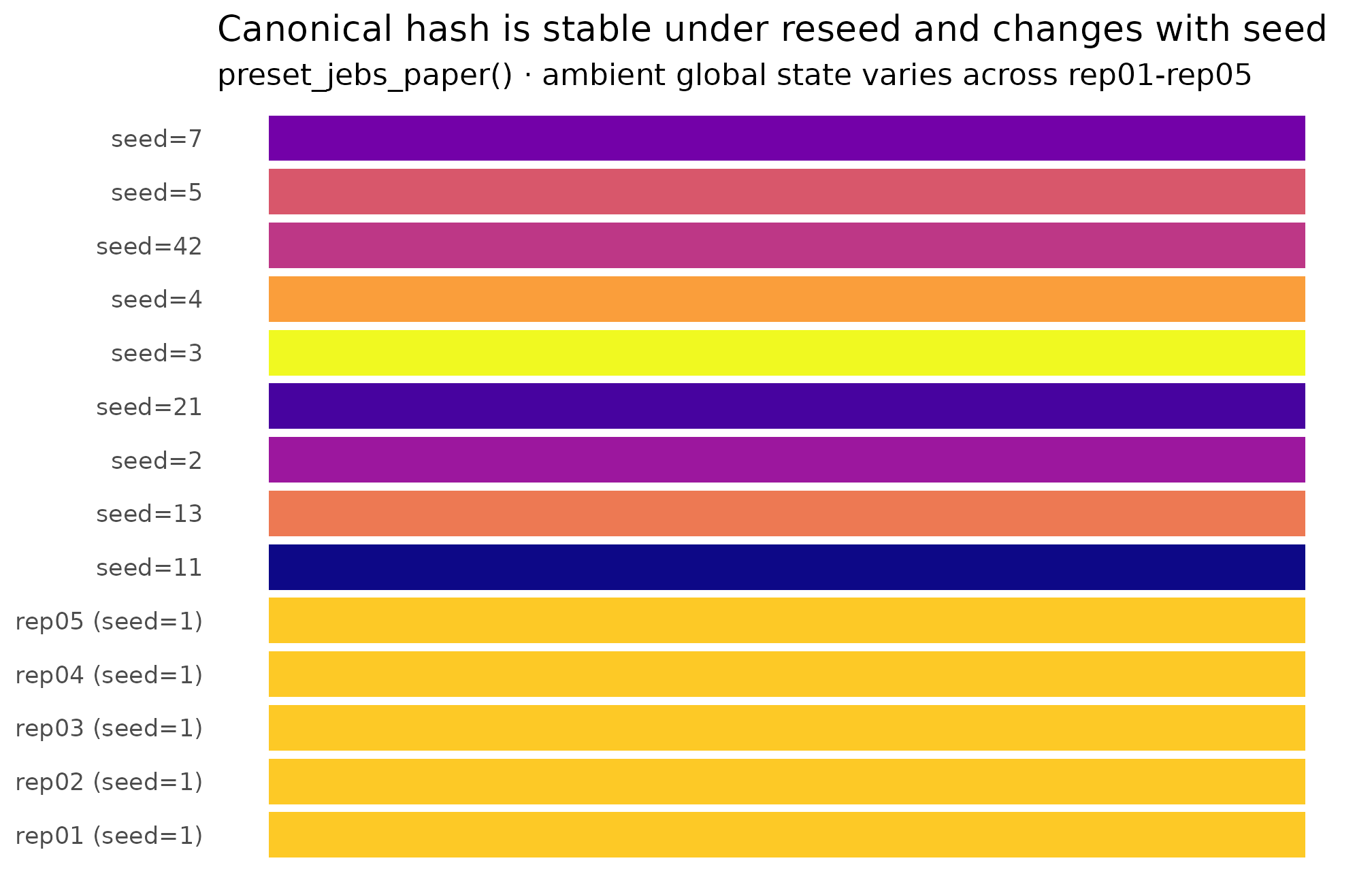
Bar chart of canonical hashes; the first five bars all show the same hash from repeated seed = 1L calls under scrambled global RNG state, while the next nine bars each show a distinct hash from a different seed value.

Each bar is one canonical hash. Five repeats of seed = 1L (scrambled global state between calls) collapse to a single hash, confirming the local-seed-stream policy. Nine different seeds give nine different hashes, confirming the seed argument is the lever.

Two things to read off the plot. First, the five rep01-rep05 bars (top of the panel) all have the same fill colour: same hash, even though the ambient global RNG was scrambled before each call. This is the local-seed-stream policy at work — the only thing that matters for canonical_hash(dat) is the value passed to the seed argument and the design ingredients. Second, the nine seed-varied bars (bottom of the panel) each have their own fill colour: a different seed gives a different hash, as expected.

5. The reproducibility contract

The package guarantees a precise statement, which is worth writing out as a contract. Given:

the same package version of multisiteDGP (the 0.1.0 line in the provenance string),
the same seed passed as the seed argument to a primary call (sim_multisite(), sim_meta(), gen_effects(), gen_observations()),
the same design (the same preset call, or the same multisitedgp_design() arguments, or the same update_multisitedgp_design() patch),

the package guarantees:

the same canonical_hash(dat) byte-for-byte,
and therefore the same realized point estimates, the same realized standard errors, the same diagnostics in the canonical allowlist, and the same provenance_string(dat) modulo the R version slot.

That is the contract. The hash is the witness. If the contract holds, two researchers running the same line of code on different machines see the same simulation, full stop. The smoke check used throughout the package documentation — sim_multisite(preset_jebs_paper(), seed = 1L) produces hash c52e75f276d82836 — is a single instance of the contract. If your local rerun matches that hash, the package install you have is in sync with the published baseline.

The contract is intentionally narrow. It is not a guarantee that:

your post-simulation analysis pipeline (a Bayesian model fit, a bootstrap, a robustness sweep) is reproducible — that is your pipeline’s responsibility, and a separate hash on the downstream artifact is the right tool there;
a different platform or a different R minor version produces the same hash — see Section 6;
a custom g_fn callback gives the same hash if you change its body — the package records callback presence, not body identity, by design (changing the body is a meaningful change to the simulation that the user should re-pin manually).

The narrowness is deliberate. A wider contract would be either unenforceable (downstream pipelines vary too much) or false (cross-platform byte-equality is not a property the package can deliver — see below).

6. What can break the contract

There are three classes of contract break, in roughly decreasing order of frequency.

6.1 Changing the package version

This is by far the most common. multisiteDGP 0.1.x → 0.2.x is a minor bump that may add fields to the canonical-hash payload, change the order in which diagnostics are computed, or alter a generator’s internal sampling scheme. Any of these legitimately changes the hash. The mitigation is the manifest: when you save pkg_version = "0.1.0" alongside the hash, a future you whose packageVersion("multisiteDGP") returns 0.2.0 knows immediately why the hashes differ, and can decide whether to install the older version (via remotes::install_version() or renv) or to re-pin the artifact at the new version. Either choice is principled; what is not principled is a silent mismatch.

6.2 Changing the R version

R version drift is rarer in practice but does occur. R 4.4 → R 4.5 changed the default RNG kind for sample.int() in some edge cases (RNGkind("Rounding") legacy behavior), and a major- version bump (R 4.x → R 5.x) is a near-certain hash break. The package emits a warning when a saved provenance string was generated under a different R version than the current session.

The provenance string carries the R version as the R=4.5 slot specifically so this is grep-able. If you see two provenance lines that differ only in the R=... slot, you have located the cause.

6.3 Changing the OS or the platform

Cross-platform hash equality is held to a weaker standard. Linux x86_64 / amd64 is the strict baseline used for the package’s golden fixtures in tests/testthat/. macOS and Windows are held to same-machine reproducibility plus distributional parity against the Linux baseline — the realized distribution of point estimates and SEs matches Linux to numerical tolerance, but the exact canonical_hash is allowed to drift because of platform-level floating-point differences in BLAS / LAPACK and compiler math libraries. The full installed policy is in system.file("REPRODUCIBILITY.md", package = "multisiteDGP"). If you and a coauthor on different operating systems produce different hashes for the same seed and design, the next check is whether the distributions of tau_j_hat and se_j agree to numerical tolerance, not the 16 hex characters.

6.4 What does not break the contract

Some things look like they should change the hash but do not. The ambient global RNG state at the moment of the call does not (see Section 4). Reordering tibble columns does not (canonicalization sorts columns). Adding a non-numeric diagnostic does not (the allowlist is numeric-only). The current working directory and the system locale do not. Knowing what is not in the payload is part of trusting the hash.

7. The IES Form 1 acknowledgments paragraph

The package is distributed with an acknowledgments paragraph (reproduced verbatim in the footer of every vignette) that names the funder, grant number, and standard disclaimer. M7 is the dedicated home in vignette space for explaining why the paragraph appears where it does.

The paragraph identifies the source of support: the Institute of Education Sciences, U.S. Department of Education, through Grant R305D240078 to the University of Alabama, with the standard disclaimer that the views expressed are the authors’ and do not represent the Institute’s. Every vignette reproduces the paragraph in its footer (uniform appearance, low cognitive load for the reader). M7 is the place where the role of the paragraph is discussed — funder acknowledgment is a condition of the grant and a research-integrity norm for federally funded methodological work, and the precise wording is fixed (Form 1) so it can be machine- checked across the package’s documentation surface in the release audit that greps for the grant number.

When you cite this package in a paper appendix, the courtesy is either to reproduce the acknowledgment paragraph verbatim or to cite the package’s CITATION entry and the underlying methods paper (Lee et al., 2025). The IES grant terms apply only to outputs the IES project itself produces.

8. Where to next

You now have, for any simulation you run with this package: a one-line provenance string, a 16-character canonical hash, a verification recipe, and a manifest pattern. The remaining vignettes build on this base.

Getting started — A1 §9 is the user-track entry point to provenance, with a lighter treatment of the same workflow.
Cookbook — recipe G walks an end-to-end manifest workflow inside a design_grid() power study.
Migration from siteBayes2 — re-pinning legacy siteBayes2 artifacts under the same audit trail.
canonical_hash() — argument reference, including the algo and columns_to_include arguments not used here.
provenance_string() — the S3 generic and the three methods (data, design, default).

For the methodological foundations the hash is fingerprinting, start with The two-stage DGP and proceed through M2 / M3 / M4 in order. For the empirical-Bayes context the package’s hash-pinned simulations are typically deployed in, see Walters (2024).

References

The multisiteDGP data-generating process and the JEBS preset implement the design in Lee et al. (2025). Empirical-Bayes context for the simulation studies the package is typically deployed in is collected in Walters (2024).

Acknowledgments

This research was supported by the Institute of Education Sciences, U.S. Department of Education, through Grant R305D240078 to the University of Alabama. The opinions expressed are those of the authors and do not represent views of the Institute or the U.S. Department of Education.

Session info

#> R version 4.6.0 (2026-04-24)
#> Platform: x86_64-pc-linux-gnu
#> Running under: Ubuntu 24.04.4 LTS
#> 
#> Matrix products: default
#> BLAS:   /usr/lib/x86_64-linux-gnu/openblas-pthread/libblas.so.3 
#> LAPACK: /usr/lib/x86_64-linux-gnu/openblas-pthread/libopenblasp-r0.3.26.so;  LAPACK version 3.12.0
#> 
#> locale:
#>  [1] LC_CTYPE=C.UTF-8       LC_NUMERIC=C           LC_TIME=C.UTF-8       
#>  [4] LC_COLLATE=C.UTF-8     LC_MONETARY=C.UTF-8    LC_MESSAGES=C.UTF-8   
#>  [7] LC_PAPER=C.UTF-8       LC_NAME=C              LC_ADDRESS=C          
#> [10] LC_TELEPHONE=C         LC_MEASUREMENT=C.UTF-8 LC_IDENTIFICATION=C   
#> 
#> time zone: UTC
#> tzcode source: system (glibc)
#> 
#> attached base packages:
#> [1] stats     graphics  grDevices utils     datasets  methods   base     
#> 
#> other attached packages:
#> [1] ggplot2_4.0.3      multisiteDGP_0.1.1
#> 
#> loaded via a namespace (and not attached):
#>  [1] gtable_0.3.6       jsonlite_2.0.0     dplyr_1.2.1        compiler_4.6.0    
#>  [5] tidyselect_1.2.1   jquerylib_0.1.4    systemfonts_1.3.2  scales_1.4.0      
#>  [9] textshaping_1.0.5  yaml_2.3.12        fastmap_1.2.0      R6_2.6.1          
#> [13] labeling_0.4.3     generics_0.1.4     knitr_1.51         tibble_3.3.1      
#> [17] desc_1.4.3         bslib_0.10.0       pillar_1.11.1      RColorBrewer_1.1-3
#> [21] rlang_1.2.0        utf8_1.2.6         cachem_1.1.0       xfun_0.57         
#> [25] fs_2.1.0           sass_0.4.10        S7_0.2.2           viridisLite_0.4.3 
#> [29] cli_3.6.6          pkgdown_2.2.0      withr_3.0.2        magrittr_2.0.5    
#> [33] digest_0.6.39      grid_4.6.0         lifecycle_1.0.5    vctrs_0.7.3       
#> [37] evaluate_1.0.5     glue_1.8.1         farver_2.1.2       ragg_1.5.2        
#> [41] rmarkdown_2.31     tools_4.6.0        pkgconfig_2.0.3    htmltools_0.5.9

Lee, J., Che, J., Rabe-Hesketh, S., Feller, A., & Miratrix, L. (2025). Improving the estimation of site-specific effects and their distribution in multisite trials. Journal of Educational and Behavioral Statistics, 50(5), 731–764. https://doi.org/10.3102/10769986241254286

Walters, C. (2024). Empirical bayes methods in labor economics. In Handbook of labor economics (Vol. 5, pp. 183–260). Elsevier. https://doi.org/10.1016/bs.heslab.2024.11.001

M7 · Reproducibility and provenance

JoonHo Lee

2026-05-10

1. Why reproducibility matters

2. The four-piece kit

3. Workflow walkthrough — pinning a single artifact

3.1 Step 1 — set the seed

3.2 Step 2 — run the simulation and capture `provenance_string()`

3.3 Step 3 — capture `canonical_hash()` separately

3.4 Step 4 — save a manifest

3.5 Step 5 — verify the hash on rerun

4. Hash stability under reseed — a visual check

5. The reproducibility contract

6. What can break the contract

6.1 Changing the package version

6.2 Changing the R version

6.3 Changing the OS or the platform

6.4 What does not break the contract

7. The IES Form 1 acknowledgments paragraph

8. Where to next

References

Acknowledgments

Session info

M7 · Reproducibility and provenance

JoonHo Lee

2026-05-10

1. Why reproducibility matters

2. The four-piece kit

3. Workflow walkthrough — pinning a single artifact

3.1 Step 1 — set the seed

3.2 Step 2 — run the simulation and capture provenance_string()

3.3 Step 3 — capture canonical_hash() separately

3.4 Step 4 — save a manifest

3.5 Step 5 — verify the hash on rerun

4. Hash stability under reseed — a visual check

5. The reproducibility contract

6. What can break the contract

6.1 Changing the package version

6.2 Changing the R version

6.3 Changing the OS or the platform

6.4 What does not break the contract

7. The IES Form 1 acknowledgments paragraph

8. Where to next

References

Acknowledgments

Session info

3.2 Step 2 — run the simulation and capture `provenance_string()`

3.3 Step 3 — capture `canonical_hash()` separately