A2 · Choosing a preset • multisiteDGP

Abstract

For researchers who know they need a multisite or meta-analytic simulation but do not yet know which preset matches their study. This vignette is a scannable decision table over the nine built-in presets — read down the rows, find your scenario, lift the call. You leave with the preset name that fits, the source citation behind it, the override pattern for adapting it to a local design, and a provenance string suitable for a methods appendix.

1. The problem with picking parameters by feel

A multisite simulation has roughly a dozen knobs that interact: $J$ , $\sigma_\tau$ , $\bar n_j$ , the latent G shape, the dependence target, the engine. Pick them one at a time and the realized design rarely matches what you intended — the implied informativeness $I$ is too high, the heterogeneity ratio $R$ is too narrow, the shrinkage flag fires unexpectedly. A preset packages a defensible combination tied to a published reference or a documented benchmark. You start there, then override the one or two fields your study departs on.

The package ships nine presets across two front doors. Seven are site-size-driven (sampling variance comes from generated $n_j$ , used with sim_multisite()); two are direct-precision (sampling variance is set through $(I, R)$ , used with sim_meta()). The rest of this vignette is a table you read down to find the row that matches your scenario, plus the override pattern for adapting it.

2. What a preset locks for you

Every preset returns a multisitedgp_design with all four generative layers already filled in. The constructor below shows what the nine presets fix at the parameters that drive the headline diagnostics — the paradigm and engine, the site count $J$ , the between-site SD $\sigma_\tau$ , the latent G shape, the site-size mean (the site-size-driven path, Paradigm A in the package’s underlying blueprint) or the $(I, R)$ pair (the direct-precision path, Paradigm B in the same blueprint), and the citation that anchors the choice.

preset_objects <- list(
  education_small        = preset_education_small(),
  education_modest       = preset_education_modest(),
  education_substantial  = preset_education_substantial(),
  jebs_paper             = preset_jebs_paper(),
  jebs_strict            = preset_jebs_strict(),
  walters_2024           = preset_walters_2024(),
  twin_towers            = preset_twin_towers(),
  meta_modest            = preset_meta_modest(),
  small_area_estimation  = preset_small_area_estimation()
)

preset_summary <- data.frame(
  preset      = names(preset_objects),
  paradigm    = vapply(preset_objects, `[[`, character(1), "paradigm"),
  engine      = vapply(preset_objects, `[[`, character(1), "engine"),
  J           = vapply(preset_objects, `[[`, integer(1),   "J"),
  sigma_tau   = vapply(preset_objects, `[[`, numeric(1),   "sigma_tau"),
  true_dist   = vapply(preset_objects, `[[`, character(1), "true_dist"),
  nj_mean     = vapply(preset_objects, function(p) p$nj_mean %||% NA_real_, numeric(1)),
  I           = vapply(preset_objects, function(p) p$I       %||% NA_real_, numeric(1)),
  R           = vapply(preset_objects, function(p) p$R       %||% NA_real_, numeric(1)),
  row.names   = NULL,
  stringsAsFactors = FALSE
)
preset_summary
#>                  preset  paradigm    engine    J sigma_tau true_dist nj_mean
#> 1       education_small site_size A2_modern   50     0.050  Gaussian      40
#> 2      education_modest site_size A2_modern   50     0.200  Gaussian      50
#> 3 education_substantial site_size A2_modern  100     0.300  Gaussian      80
#> 4            jebs_paper site_size A1_legacy   50     0.200   Mixture      40
#> 5           jebs_strict site_size A1_legacy  100     0.150   Mixture      80
#> 6          walters_2024 site_size A2_modern   46     0.197  Gaussian     240
#> 7           twin_towers site_size A2_modern 1000     2.000   Mixture     100
#> 8           meta_modest    direct A2_modern   50     0.200  Gaussian      50
#> 9 small_area_estimation    direct A2_modern   30     0.200  Gaussian      50
#>     I   R
#> 1  NA 1.0
#> 2  NA 1.0
#> 3  NA 1.0
#> 4  NA 1.0
#> 5  NA 1.0
#> 6  NA 1.0
#> 7  NA 1.0
#> 8 0.3 1.5
#> 9 0.2 3.0

Read across a row as the locked design. The two direct-precision presets at the bottom carry the active $(I, R)$ pair that drives their sampling-variance distribution; their nj_mean field surfaces the constructor default and is not used at simulation time. The seven site-size presets above them carry the active nj_mean (and the implicit cv, nj_min, R2 settings printed by the design object itself); their $(I, R)$ entries surface constructor defaults and are not used — realized $I$ and $R$ fall out of the site-size distribution and the chosen $\sigma_\tau$ at simulation time.

The two engines you see — A1_legacy and A2_modern — produce identical numerical results on the standardized residual scale; the difference is internal plumbing. The two JEBS presets pin A1_legacy because the published JEBS results were generated under that engine and the parity check on the JEBS table requires it. Everything else uses A2_modern. See Margin and SE models for the engine discussion.

3. The decision rubric

Read this table down, top to bottom, until a row describes your study. The recommended preset is the call to lift; the locked parameters column is what that preset will fix for you; the source column is the published reference behind the calibration; the override column is the field most studies need to change first.

Scenario	Preset	Locked: J / sigma_tau / paradigm	Source	Most common override
Education trial, small effects (~0.05) on the standardized scale	`preset_education_small()`	J = 50 / 0.05 / site-size	Weiss et al. (2017)	`J`, `nj_mean`
Education trial, modest effects (~0.20) — typical RCT scale	`preset_education_modest()`	J = 50 / 0.20 / site-size	Weiss et al. (2017)	`J`, `sigma_tau`
Education trial, substantial effects (~0.30), large J	`preset_education_substantial()`	J = 100 / 0.30 / site-size	Weiss et al. (2017)	`nj_mean`
Reproduce the JEBS paper design (mixture-shape latent effects)	`preset_jebs_paper()`	J = 50 / 0.20 / site-size	Lee et al. (2025)	(none — verbatim)
JEBS strict parity grid (validation / benchmarking)	`preset_jebs_strict()`	J = 100 / 0.15 / site-size	Lee et al. (2025)	(none — verbatim)
Replicate the Walters Handbook chapter calibration	`preset_walters_2024()`	J = 46 / 0.197 / site-size; locks $R^2 = 0.4$ , $\bar n_j = 240$	Walters (2024)	`R2`
Large-J / extreme heterogeneity stress test	`preset_twin_towers()`	J = 1000 / 2.0 / site-size	Package-curated	`J`
Meta-analysis warm-up (direct-precision path)	`preset_meta_modest()`	J = 50 / 0.20 / direct; locks $I = 0.30$ , $R = 1.5$	Package-curated	`I`, `R`
Small-area-estimation prior calibration	`preset_small_area_estimation()`	J = 30 / 0.20 / direct; locks $I = 0.20$ , $R = 3$	Package-curated	`I`, `R`

Three reading rules.

First — the paradigm column is the most consequential entry. If you plan to call sim_multisite(), you need a row whose paradigm is site-size. If you plan to call sim_meta(), you need direct. Mixing them produces an immediate front-door error (Section 7).

Second — source tells you what published number you are inheriting. The three education presets share Weiss et al. (2017) as their sigma-tau anchor (Weiss et al., 2017). The two JEBS presets implement the simulation design from Lee et al. (2025). preset_walters_2024() reproduces the calibration in the Handbook of Labor Economics, volume 5 chapter by Walters (2024). The remaining three presets are package-curated rather than paper-anchored and carry no external citation.

Third — override is the field most studies change first. Education presets retain $\sigma_\tau$ but adjust $J$ to match the local sample of schools; the Walters preset retains $J$ and $\sigma_\tau$ but adjusts the covariate $R^2$ . JEBS rows show no override because their value is reproducing the published number exactly — change a JEBS field and the preset name no longer applies.

A compact tree view (alternative)

Readers who prefer branching to tabular logic can walk the same rubric as a four-question tree:

Q1 paradigm
├── multisite trial -> Q2 calibration source
│   ├── JEBS paper        -> Q3 grid
│   │   ├── paper-grid    -> preset_jebs_paper()
│   │   └── strict-grid   -> preset_jebs_strict()
│   ├── Walters Handbook  -> preset_walters_2024()
│   ├── Education applied -> Q4 effect-size scale
│   │   ├── small  ~0.05  -> preset_education_small()
│   │   ├── modest ~0.20  -> preset_education_modest()
│   │   └── subst. ~0.30  -> preset_education_substantial()
│   └── stress test       -> preset_twin_towers()
└── meta-analysis     -> Q5 special requirements
    ├── methods warm-up   -> preset_meta_modest()
    └── small-area prior  -> preset_small_area_estimation()

If a reviewer asks why a particular preset, you trace four nodes through this tree and you have your answer.

When to override versus pick a different row

If you find yourself overriding more than two fields, you are in a different row. Move to the row whose locked parameters are closest to your design, then override at most one or two. The presets are not fragile — every preset accepts named overrides through ... — but their defensibility comes from the published anchor. Overriding the sigma-tau of a Weiss-anchored preset to 0.40 silently breaks the anchor. Pick preset_education_substantial() instead and tune from there.

4. Override patterns

Overrides are flat, named arguments forwarded to the underlying multisitedgp_design() constructor. Anything you do not name is left at the preset default.

local_design <- preset_education_modest(
  J          = 20L,
  nj_mean    = 60,
  sigma_tau  = 0.25
)

local_design
#> <multisitedgp_design>
#> Paradigm: site_size    Engine: A2_modern    Framing: superpopulation
#> J: 20    Seed: NULL (active RNG)    Lifecycle: experimental
#> 
#> [ Layer 1: G-effects ]
#>   true_dist:  Gaussian
#>   tau:        0
#>   sigma_tau:  0.25
#>   formula:    NULL
#>   beta:       NULL
#>   g_fn:       NULL
#> 
#> [ Layer 2: Margin (Paradigm A) ]
#>   nj_mean:    60
#>   cv:         0.5
#>   nj_min:     10
#>   p:          0.5
#>   R2:         0
#>   var_outcome: 1
#> 
#> [ Layer 3: Dependence ]
#>   method:        none
#>   rank_corr:     0
#>   pearson_corr:  0
#>   hybrid_init:   copula
#>   hybrid_polish: hill_climb
#>   dependence_fn: NULL
#> 
#> [ Layer 4: Observation ]
#>   obs_fn: NULL
#> 
#> Use sim_multisite(design) or sim_meta(design) to simulate.

Three things to read off the printed object. The header shows $J$ moved from the preset default 50 to 20. The Layer 1 $\sigma_\tau$ moved from 0.20 to 0.25 — a modest tune-up to match a local pilot. In Layer 2 (Margin), nj_mean moved from 50 to 60. Every unnamed field — cv = 0.5, nj_min = 10, the dependence settings, the observation hook — survives untouched from the preset.

Now simulate from the override design and check that the realized diagnostics still pass:

local_dat <- sim_multisite(local_design, seed = 2027L)
summary(local_dat)
#> multisiteDGP simulation diagnostics
#> ------------------------------------------------------------
#> A. Realized vs Intended
#>    I (informativeness):         0.396  (target N/A)  N/A   [no target]
#>    R (SE heterogeneity):        4.714  (target N/A)  N/A   [no target]
#>    sigma_tau:                   0.273  (target 0.250)  WARN  [rel=9.1%]
#>    GM(se^2):                    0.095  (target N/A)  N/A   [no target]
#> 
#> B. Dependence
#>    rank_corr residual:         -0.103  (target 0.000)  PASS  [delta=-0.103]
#>    rank_corr marginal:         -0.103  (target N/A)  N/A   [residual target rows only; no finite target; status not assigned]
#>    pearson_corr residual:      -0.124  (target 0.000)  FAIL  [delta=-0.124]
#>    pearson_corr marginal:      -0.124  (target N/A)  N/A   [residual target rows only; no finite target; status not assigned]
#> 
#> C. G shape fit
#>    KS distance D_J:             0.200  (target 0.000)  PASS  [p=0.832]
#>    Bhattacharyya BC:            0.441  (target 1.000)  FAIL  [rel=-55.9%]
#>    Q-Q residual:                0.460  (target 0.000)  N/A   [delta=0.460]
#> 
#> D. Operational feasibility
#>    mean shrinkage S:            0.401  (target N/A)  PASS  [no target]
#>    avg MOE (95%):               0.623  (target N/A)  WARN  [no target]
#>    feasibility_index:           8.016  (target N/A)  WARN  [no target]
#> ------------------------------------------------------------
#> Overall: 3 PASS, 3 WARN, 2 FAIL.
#> Provenance: multisiteDGP 0.1.1 | paradigm=site_size | seed=2027 | canonical_hash=e4d3e7cabb623cf3 | design_hash=8f8485997bc6a366 | hash_algo=xxhash64 | R=4.6.0 | hooks=none

The realized $\sigma_\tau$ landed at 0.273 against the target 0.250 (WARN, $\sim 9$ percent relative drift — small-J sampling noise, not a design error). The dependence diagnostic on the rank scale passes at $-0.103$ against target zero. Operational feasibility flags WARN because $J = 20$ leaves the effective per-site sample size near 8 — expected for the small-J override.

The general override rules:

One field at a time first. Bump $\sigma_\tau$ , re-render, check the diagnostics. Only move on if the realized values look right.
Re-render summary() after every override. A field move can push a previously-passing diagnostic into WARN.
Document the override in your provenance string. The canonical_hash() and provenance_string() carry the override into the methods appendix automatically — you do not need to spell out the field changes in prose.

5. Visual comparison across presets

A scannable table loses one piece of context: how the realized site effects actually look across presets. The plot below pulls three presets covering the heterogeneity range — small (Weiss low end), modest (JEBS / Weiss middle), and substantial (Weiss upper, large J) — and overlays their $\widehat\tau_j$ distributions on a common axis.

ggplot2::ggplot(
  compare_df,
  ggplot2::aes(x = factor(preset, levels = c("education_small",
                                             "education_modest",
                                             "education_substantial")),
               y = tau_hat)
) +
  ggplot2::geom_jitter(width = 0.18, alpha = 0.55, size = 1.4) +
  ggplot2::geom_hline(
    data    = unique(compare_df[, c("preset", "sigma_tau")]),
    mapping = ggplot2::aes(yintercept = sigma_tau),
    linetype = "dashed", color = "grey45"
  ) +
  ggplot2::geom_hline(
    data    = unique(compare_df[, c("preset", "sigma_tau")]),
    mapping = ggplot2::aes(yintercept = -sigma_tau),
    linetype = "dashed", color = "grey45"
  ) +
  ggplot2::labs(
    x        = NULL,
    y        = expression(hat(tau)[j]),
    title    = "Site-effect spread across three education presets",
    subtitle = "Dashed lines mark each preset's sigma_tau target"
  ) +
  ggplot2::theme_minimal(base_size = 11)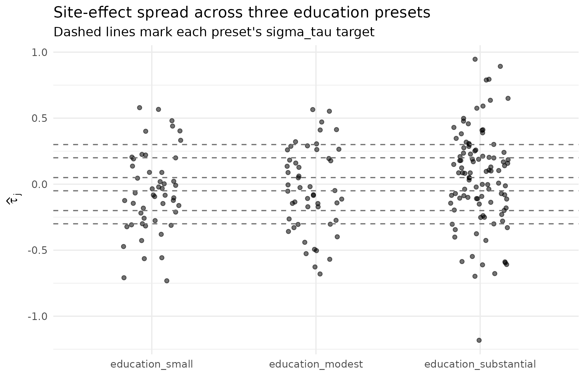

Three side-by-side strip plots of observed site effects across the three Weiss-anchored education presets, showing increasing vertical spread as sigma_tau grows.

Realized observed estimates across three Weiss-anchored presets at seed = 1L. Vertical spread widens as the preset’s sigma_tau grows (0.05, 0.20, 0.30 — left to right). The fixed sigma_tau anchor of each preset is the dashed reference line. The small-effects column’s cloud nearly collapses to zero because the latent SD is small relative to sampling error; the substantial column’s cloud is widest, with J = 100 narrowing each site’s bar and pulling the cloud closer to its dashed band.

What to read off this plot, in this order.

Vertical spread. The substantial-effects column should be visibly wider than the modest and small columns; that is the $\sigma_\tau$ ladder you locked in by choosing one preset over another.
Bar density at the dashed lines. Roughly two-thirds of the site dots should fall inside each preset’s $\pm \sigma_\tau$ band — the empirical rule for an SD-scale parameter.
The small column collapsing. When $\sigma_\tau = 0.05$ , latent variation is dominated by sampling noise; the dots scatter widely relative to the dashed band. That is the calibration warning preset_education_small() is meant to make explicit, not a bug in the preset.

6. Diagnostic per preset — funnel for `preset_jebs_paper()`

The visual contract for an individual preset is its funnel plot. Below is the funnel for preset_jebs_paper() — the rank-correlation target is zero, so a symmetric scatter top-to-bottom is the expected signature. If the cloud tilts, the design has accidentally induced precision–effect dependence and the rank-correlation diagnostic in Group B will flip from PASS to FAIL.

dat_jebs <- sim_multisite(preset_jebs_paper(), seed = 1L)
plot_funnel(dat_jebs, caption = FALSE) +
  ggplot2::labs(
    title    = "preset_jebs_paper() — funnel diagnostic",
    subtitle = "Symmetric cloud confirms rho_S target = 0"
  )

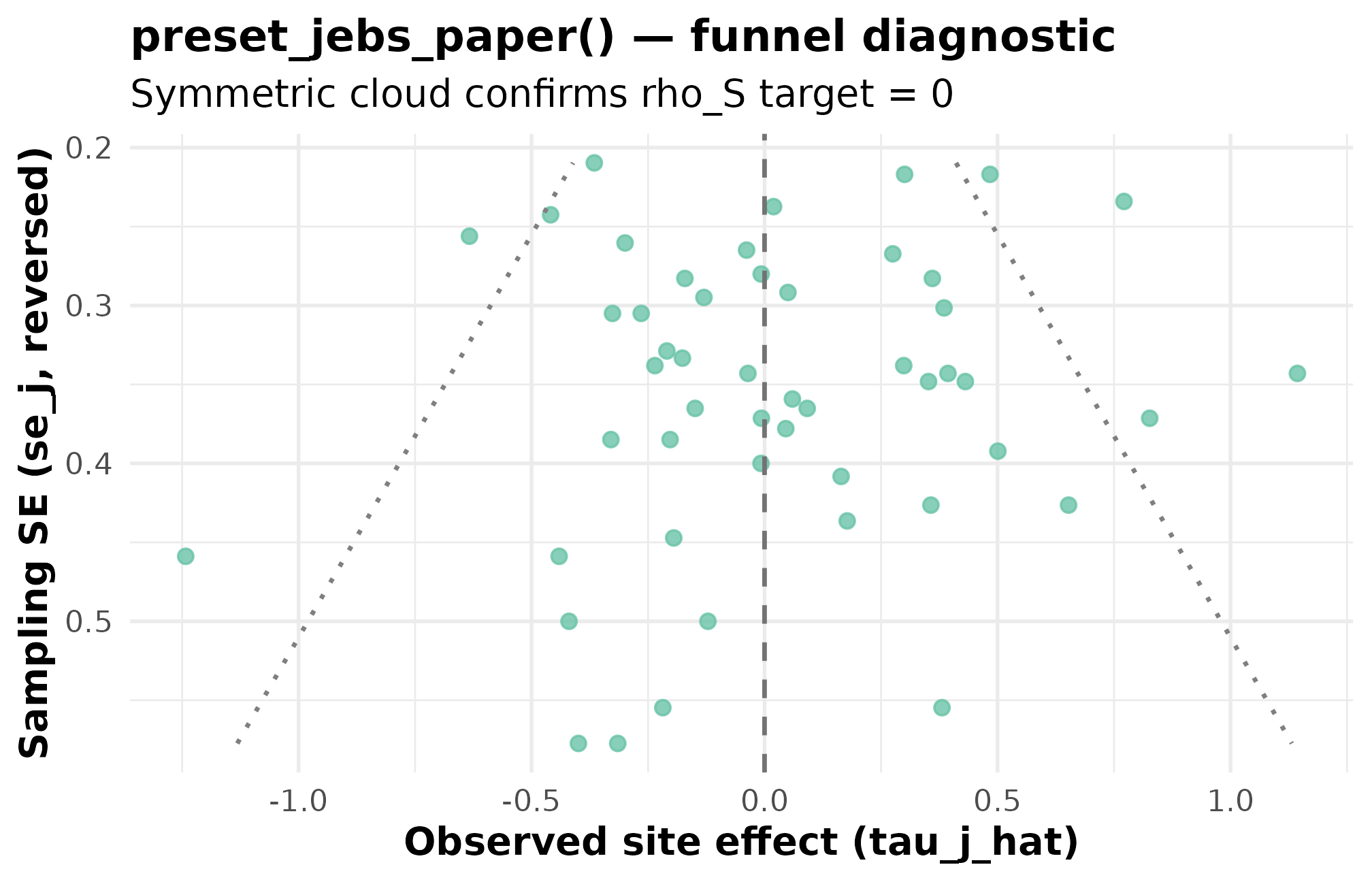
Funnel plot for preset_jebs_paper showing the standard error on the x-axis and observed estimate on the y-axis, with roughly symmetric scatter around zero.

Funnel plot for preset_jebs_paper() at seed = 1L. Standard error on the x-axis (smaller = more precise); observed estimate on the y-axis. The cloud tapers as SE shrinks because the design generates SE from site sizes — the funnel signature of the site-size-driven path. Symmetry top-to-bottom confirms the rank-correlation target rho_S = 0 (PASS at -0.193, well within sampling tolerance for J = 50).

The same visual contract applies to every site-size preset; only the spread and the funnel-mouth width change. For preset_education_small() the cloud is narrower vertically; for preset_twin_towers() it is enormous (J = 1000, $\sigma_\tau = 2$ ). The diagnostic question — “is the cloud symmetric around zero” — stays identical. See Diagnostics in practice for the full four-group rubric.

7. Wrong-door checks

Front doors are intentionally strict. A site-size preset belongs to sim_multisite(), and a direct-precision preset belongs to sim_meta(). Mixing them produces a clean error rather than a silent miscalculation.

tryCatch(
  sim_meta(preset_education_modest(), seed = 1L),
  error = function(e) conditionMessage(e)
)
#> [1] "\033[1m\033[22m\033[31m✖\033[39m `sim_meta()` requires `paradigm = \"direct\"`.\n\033[36mℹ\033[39m Got `design$paradigm = \"site_size\"`.\n→ Use `sim_multisite()` for site-size designs."

Read the error: the wrapper says it requires paradigm = "direct", notes the design carried paradigm = "site_size", and points you to the right front door. Reverse the example and the same guard fires the other way.

The second wrong-door check is a calibration FAIL inside a preset that the user picked at the wrong scale. If Maya picks preset_education_small() ( $\sigma_\tau = 0.05$ ) for a study whose real heterogeneity is closer to 0.20, the simulation runs without error — but the diagnostics catch it.

small_dat <- sim_multisite(preset_education_small(), seed = 1L)
summary(small_dat)
#> multisiteDGP simulation diagnostics
#> ------------------------------------------------------------
#> A. Realized vs Intended
#>    I (informativeness):         0.021  (target N/A)  N/A   [no target]
#>    R (SE heterogeneity):       12.125  (target N/A)  N/A   [no target]
#>    sigma_tau:                   0.042  (target 0.050)  FAIL  [rel=-16.9%]
#>    GM(se^2):                    0.116  (target N/A)  N/A   [no target]
#> 
#> B. Dependence
#>    rank_corr residual:          0.261  (target 0.000)  PASS  [delta=0.261]
#>    rank_corr marginal:          0.261  (target N/A)  N/A   [residual target rows only; no finite target; status not assigned]
#>    pearson_corr residual:       0.386  (target 0.000)  FAIL  [delta=0.386]
#>    pearson_corr marginal:       0.386  (target N/A)  N/A   [residual target rows only; no finite target; status not assigned]
#> 
#> C. G shape fit
#>    KS distance D_J:             0.140  (target 0.000)  PASS  [p=0.717]
#>    Bhattacharyya BC:            0.801  (target 1.000)  WARN  [rel=-19.9%]
#>    Q-Q residual:                0.731  (target 0.000)  N/A   [delta=0.731]
#> 
#> D. Operational feasibility
#>    mean shrinkage S:            0.024  (target N/A)  FAIL  [no target]
#>    avg MOE (95%):               0.697  (target N/A)  FAIL  [no target]
#>    feasibility_index:           1.188  (target N/A)  FAIL  [no target]
#> ------------------------------------------------------------
#> Overall: 2 PASS, 1 WARN, 5 FAIL.
#> Provenance: multisiteDGP 0.1.1 | paradigm=site_size | seed=1 | canonical_hash=209d790e83aa6976 | design_hash=caae328a59a97738 | hash_algo=xxhash64 | R=4.6.0 | hooks=none

Read the diagnostics. The realized $\sigma_\tau$ comes in at 0.042 against a target of 0.050 — that is a FAIL, even though the small-J ( $J = 50$ ) sampling noise is the dominant cause. The implied operational feasibility flag at the bottom (mean shrinkage, average MOE, feasibility index) fires a red status because the latent signal is small relative to sampling error. The simulation ran cleanly — it is the design that is wrong for this scenario. Switch to preset_education_modest() and the same diagnostics return to PASS or WARN territory at appropriate magnitudes.

8. Defending the choice

Once a preset is selected and any overrides are applied, the provenance string carries the choice and the seed into the methods appendix in one line.

chosen_dat <- sim_multisite(preset_jebs_paper(), seed = 1L)
provenance_string(chosen_dat)
#> [1] "multisiteDGP 0.1.1 | paradigm=site_size | seed=1 | canonical_hash=b29561b47a40332d | design_hash=cddffb66364a11ee | hash_algo=xxhash64 | R=4.6.0 | hooks=none"

The string contains the package version, the paradigm, the seed, the canonical hash of the simulation, the design hash, the hashing algorithm, the R version, and any active hooks. Pasting this into a methods appendix gives a reviewer the exact contract: identical package version + identical seed + identical preset → identical canonical hash → byte-identical simulation. The hash itself is the short anchor:

canonical_hash(chosen_dat)
#> [1] "b29561b47a40332d"

Cite the source for the chosen preset in prose. For preset_jebs_paper() and preset_jebs_strict() cite Lee et al. (2025); for preset_walters_2024() cite Walters (2024); for the three education presets cite Weiss et al. (2017). The three remaining presets are package-curated and carry no external citation; describe each by role (“a stress-test preset for J = 1000 with extreme heterogeneity”; “a meta-analysis warm-up at the direct-precision front door”; “a small-area-estimation prior calibration”) rather than naming a paper.

A reviewer-ready methods-appendix line ties it all together:

Simulation generated with multisiteDGP (version 0.1.0, Lee 2025) using preset_education_modest(J = 20L, nj_mean = 60, sigma_tau = 0.25), seed = 2027L, canonical hash 4f9399b626d1c71f.

Three lines, every load-bearing claim grounded in either a citation or a hash.

9. Where to next

A1 · Getting started — if you have not already run a first simulation end-to-end, start there.
Diagnostics in practice — the four diagnostic groups and the plots that go with each.
Covariates and precision dependence — for the R2 override on preset_walters_2024() and how precision–effect dependence enters Layer 3.
Calibrating to real data — when you have observed point estimates and SEs you want the simulator to match.
Cookbook — recipe walkthroughs for downstream analysis on a fitted preset.

For methodology — the formal two-stage DGP, the G-distribution catalog, the site-size-driven and direct-precision paths — start with The two-stage DGP and read M2 / M3 / M4 in order.

References

The three education presets inherit their $\sigma_\tau$ ladder from Weiss et al. (2017). The two JEBS presets reproduce the simulation design in Lee et al. (2025). preset_walters_2024() is calibrated to the Handbook chapter Walters (2024). The remaining three presets — preset_meta_modest(), preset_small_area_estimation(), preset_twin_towers() — are package-curated and carry no published anchor at this writing.

Acknowledgments

This research was supported by the Institute of Education Sciences, U.S. Department of Education, through Grant R305D240078 to the University of Alabama. The opinions expressed are those of the authors and do not represent views of the Institute or the U.S. Department of Education.

Session info

#> R version 4.6.0 (2026-04-24)
#> Platform: x86_64-pc-linux-gnu
#> Running under: Ubuntu 24.04.4 LTS
#> 
#> Matrix products: default
#> BLAS:   /usr/lib/x86_64-linux-gnu/openblas-pthread/libblas.so.3 
#> LAPACK: /usr/lib/x86_64-linux-gnu/openblas-pthread/libopenblasp-r0.3.26.so;  LAPACK version 3.12.0
#> 
#> locale:
#>  [1] LC_CTYPE=C.UTF-8       LC_NUMERIC=C           LC_TIME=C.UTF-8       
#>  [4] LC_COLLATE=C.UTF-8     LC_MONETARY=C.UTF-8    LC_MESSAGES=C.UTF-8   
#>  [7] LC_PAPER=C.UTF-8       LC_NAME=C              LC_ADDRESS=C          
#> [10] LC_TELEPHONE=C         LC_MEASUREMENT=C.UTF-8 LC_IDENTIFICATION=C   
#> 
#> time zone: UTC
#> tzcode source: system (glibc)
#> 
#> attached base packages:
#> [1] stats     graphics  grDevices utils     datasets  methods   base     
#> 
#> other attached packages:
#> [1] ggplot2_4.0.3      multisiteDGP_0.1.1
#> 
#> loaded via a namespace (and not attached):
#>  [1] gtable_0.3.6       jsonlite_2.0.0     dplyr_1.2.1        compiler_4.6.0    
#>  [5] tidyselect_1.2.1   nleqslv_3.3.7      jquerylib_0.1.4    systemfonts_1.3.2 
#>  [9] scales_1.4.0       textshaping_1.0.5  yaml_2.3.12        fastmap_1.2.0     
#> [13] R6_2.6.1           labeling_0.4.3     generics_0.1.4     knitr_1.51        
#> [17] tibble_3.3.1       desc_1.4.3         bslib_0.10.0       pillar_1.11.1     
#> [21] RColorBrewer_1.1-3 rlang_1.2.0        cachem_1.1.0       xfun_0.57         
#> [25] fs_2.1.0           sass_0.4.10        S7_0.2.2           cli_3.6.6         
#> [29] pkgdown_2.2.0      withr_3.0.2        magrittr_2.0.5     digest_0.6.39     
#> [33] grid_4.6.0         lifecycle_1.0.5    vctrs_0.7.3        evaluate_1.0.5    
#> [37] glue_1.8.1         farver_2.1.2       ragg_1.5.2         rmarkdown_2.31    
#> [41] tools_4.6.0        pkgconfig_2.0.3    htmltools_0.5.9

Lee, J., Che, J., Rabe-Hesketh, S., Feller, A., & Miratrix, L. (2025). Improving the estimation of site-specific effects and their distribution in multisite trials. Journal of Educational and Behavioral Statistics, 50(5), 731–764. https://doi.org/10.3102/10769986241254286

Walters, C. (2024). Empirical bayes methods in labor economics. In Handbook of labor economics (Vol. 5, pp. 183–260). Elsevier. https://doi.org/10.1016/bs.heslab.2024.11.001

Weiss, M. J., Bloom, H. S., Verbitsky-Savitz, N., Gupta, H., Vigil, A. E., & Cullinan, D. N. (2017). How much do the effects of education and training programs vary across sites? Evidence from past multisite randomized trials. Journal of Research on Educational Effectiveness, 10(4), 843–876. https://doi.org/10.1080/19345747.2017.1300719

A2 · Choosing a preset

JoonHo Lee

2026-05-10

1. The problem with picking parameters by feel

2. What a preset locks for you

3. The decision rubric

A compact tree view (alternative)

When to override versus pick a different row

4. Override patterns

5. Visual comparison across presets

6. Diagnostic per preset — funnel for `preset_jebs_paper()`

7. Wrong-door checks

8. Defending the choice

9. Where to next

References

Acknowledgments

Session info

A2 · Choosing a preset

JoonHo Lee

2026-05-10

1. The problem with picking parameters by feel

2. What a preset locks for you

3. The decision rubric

A compact tree view (alternative)

When to override versus pick a different row

4. Override patterns

5. Visual comparison across presets

6. Diagnostic per preset — funnel for preset_jebs_paper()

7. Wrong-door checks

8. Defending the choice

9. Where to next

References

Acknowledgments

Session info

6. Diagnostic per preset — funnel for `preset_jebs_paper()`