M2 · G-distribution catalog and standardization

JoonHo Lee

2026-05-10

Abstract

For methodologists and reviewers who need to know exactly which shape of latent-effect distribution multisiteDGP is putting under the simulation, and exactly how that shape is rescaled before it reaches the rest of the pipeline. This vignette is organized one section per shape: each of the eight built-in G distributions gets its own parameterization, density, unit-variance derivation, generator function, and decision rule for when to use it. You leave with eight density-and-QQ panels, a sanity table of realized var(z_j) at J = 200, and a decision rubric for picking among Student-t, skew-normal, and the asymmetric Laplace.

1. Why standardization matters

The two-stage data-generating process documented in M1: The two-stage DGP factors the latent site effect as

$$\tau_j \;=\; \tau \;+\; \sigma_\tau \cdot z_j, \qquad z_j \sim G_0(\boldsymbol\theta_G), \qquad E[z_j] = 0, \;\; \mathrm{Var}(z_j) = 1.$$

The factorization splits the cross-site distribution into two ingredients. The shape of $G$ — Gaussian, Student-t, skew-normal, asymmetric Laplace, two-component mixture, point-mass-plus-slab, user-supplied callback, or Dirichlet-process-mixture stub — lives in the standardized residual $z_j$ and is parameterized by $\boldsymbol\theta_G$. The scale of the cross-site spread lives in the multiplier $\sigma_\tau$. The package keeps the two strictly separate by enforcing $\mathrm{Var}(z_j) = 1$ inside the generator. Every shape in the catalog is rescaled to unit variance before it leaves the Layer-1 generator [blueprint Ch. 5 §0]; the only place $\sigma_\tau$ is multiplied in is the location-scale wrapper above.

Why this convention matters. Without it, a non-Gaussian shape’s intrinsic variance and the user-supplied $\sigma_\tau$ are confounded: asking for “Student-$t$ with $\sigma_\tau = 0.25$” can silently produce cross-site SDs near $0.25 \cdot \sqrt{\nu/(\nu - 2)}$ rather than $0.25$. The companion JEBS-paper-era package siteBayes2 had exactly this double-scaling pattern: the legacy gen_priorG2 would draw from shape-specific densities whose own variance was not 1, then multiply by $\sigma_\tau$ a second time. The fix in multisiteDGP is the unit-variance convention enforced shape-by-shape, with the standardization done analytically wherever closed forms exist (Gaussian, Student-t, skew-normal, asymmetric Laplace) and verified numerically where they do not (the two-component mixture, the point-mass-plus-slab, and any user callback).

A second payoff matters for empirical work. Because shape and scale are decoupled, the informativeness scalar (Lee et al., 2025) depends on $\boldsymbol\theta_G$ only through $\sigma_\tau$, so empirical-Bayes shrinkage diagnostics (Walters, 2024) compare like-with-like across shapes.

2. The catalog at a glance

The eight shapes the package supports, with their theta_G fields and their canonical use cases. The order matches the rest of the vignette; the exported Layer-1 generator name is given in code font.

Shape	true_dist	theta_G fields	Layer-1 generator	Reach for it when
Gaussian	"Gaussian"	(none)	gen_effects_gaussian()	You have no prior reason to depart from normality — the JEBS default.
Student-t	"StudentT"	nu (numeric > 2)	gen_effects_studentt()	Heavy tails matter (a few sites with extreme effects).
Skew-normal	"SkewN"	slant (numeric)	gen_effects_skewn()	One-sided skew is plausible (program-effect tails).
ALD	"ALD"	rho (in (0, 1))	gen_effects_ald()	Skewness with sharper peaks; quantile interpretation.
Mixture	"Mixture"	delta, eps, ups	gen_effects_mixture()	Bimodality, contamination, latent classes of sites.
Point-mass-plus-slab	"PointMassSlab"	pi0, plus slab params	gen_effects_pmslab()	A fraction of sites are exactly null (sparse effects).
User	"User"	(whatever your callback consumes)	gen_effects_user()	None of the seven match — bring your own generator.
DPM	"DPM"	(deferred)	gen_effects_dpm()	Use the User bridge — built-in DPM sampling is deferred.

The first six are the closed-catalog choices. User is the escape hatch — supply a function that returns a length-J numeric vector, and the package treats it as a standardized residual generator (Convention A — the recommended path; mean 0, variance 1) or as a final-effect generator (Convention B — the wrapper bypass; less common). DPM is a placeholder: the public surface accepts the string for forward compatibility, but a built-in Dirichlet-process sampler is deferred to a later release. Calling true_dist = "DPM" without a g_fn bridge is rejected with an actionable error (see Section 3.8).

3. Per-shape sections

Each of the eight subsections below follows the same template: parameterization, formal density, unit-variance derivation, the exported Layer-1 generator, when to reach for the shape, and a density / QQ-against-Gaussian panel. A reader can jump straight to the shape they need without reading the others — this is the “organize-by-shape” view; the cross-shape audit lives at Section 4.

3.1 Gaussian

Parameterization. None: $\boldsymbol\theta_G = \emptyset$. The shape is fully specified by location $\tau$ and scale $\sigma_\tau$ in the wrapper.

Density. $z_j \sim \mathcal{N}(0, 1)$, with density

$$\phi(z) \;=\; \frac{1}{\sqrt{2\pi}} \exp\bigl(-z^2 / 2\bigr).$$

Unit-variance derivation. Trivial: $E[z_j] = 0$ and $\mathrm{Var}(z_j) = 1$ by construction. No rescaling.

Identifiability. The map $(\tau, \sigma_\tau) \mapsto \mathcal{N}(\tau, \sigma_\tau^2)$ is one-to-one for $\sigma_\tau > 0$.

Generator. gen_effects_gaussian() — no shape arguments beyond J, tau, and sigma_tau. Equivalent to the gen_effects() entry point with true_dist = "Gaussian" (the default).

When to reach for it. This is the JEBS-paper default (Lee et al., 2025). Most applied multisite trials at $J \le 50$ cannot empirically distinguish Gaussian from a mild Student-t or skew-normal anyway, so the default is rarely wrong as a first pass.

set.seed(1L)
out_gaussian <- gen_effects(
  J         = 200L,
  tau       = 0,
  sigma_tau = 1,
  true_dist = "Gaussian",
  theta_G   = list()
)
summary(out_gaussian$z_j)
#>     Min.  1st Qu.   Median     Mean  3rd Qu.     Max. 
#> -2.21470 -0.61383 -0.04937  0.03554  0.61300  2.40162
var(out_gaussian$z_j)
#> [1] 0.8632217

The realized variance lands close to 1 — the small departure is sampling fluctuation at $J = 200$, not a standardization defect.

3.2 Student-t

Parameterization. $\boldsymbol\theta_G = \{\nu\}$ with $\nu > 2$ (degrees of freedom). The strict inequality is the package contract: the variance of a $t_\nu$ is $\nu / (\nu - 2)$, which diverges at $\nu = 2$ and is undefined for $\nu \le 2$. Standardizing requires a finite second moment, so $\nu \le 2$ is rejected at construction.

Density. Standard Student-$t$ on $\nu$ degrees of freedom, then rescaled so the variance equals 1:

$$T \sim t_\nu, \qquad z_j \;=\; T \cdot \sqrt{\frac{\nu - 2}{\nu}}.$$

Unit-variance derivation. $\mathrm{Var}(T) = \nu / (\nu - 2)$ implies $\mathrm{Var}(z_j) = (\nu - 2)/\nu \cdot \nu/(\nu - 2) = 1$ exactly.

Identifiability. Hard refuse $\nu \le 2$ (variance non-finite); soft warn at $\nu < 4$ (kurtosis non-finite, sample-variance estimates unstable on small $J$).

Generator. gen_effects_studentt() — required theta_G$nu; the closed-form rescaler is applied internally.

When to reach for it. Heavy-tailed effects — a few sites with substantively large effects relative to the bulk; robustness checks of empirical-Bayes shrinkage estimators (Walters, 2024). The package convention is $\nu = 5$ (variance and kurtosis both finite).

set.seed(1L)
out_studentt <- gen_effects(
  J         = 200L,
  tau       = 0,
  sigma_tau = 1,
  true_dist = "StudentT",
  theta_G   = list(nu = 5)
)
summary(out_studentt$z_j)
#>       Min.    1st Qu.     Median       Mean    3rd Qu.       Max. 
#> -3.2726320 -0.5608631 -0.0770248  0.0006215  0.4530704  5.4278224
var(out_studentt$z_j)
#> [1] 1.019028

Asking for theta_G = list() (no nu) returns an actionable error that names the missing field and the canonical fix:

set.seed(1L)
gen_effects(J = 200L, tau = 0, sigma_tau = 1,
            true_dist = "StudentT", theta_G = list())
#> Error in `.abort_multisitedgp()`:
#> ✖ `theta_G` must be a named list.
#> ℹ Distribution-specific parameters are read by name.
#> → Pass `theta_G = list(...)` with named entries.

3.3 Skew-Normal

Parameterization. $\boldsymbol\theta_G = \{\alpha\}$ with $\alpha \in \mathbb{R}$ — the slant in the Azzalini parameterization (Azzalini, 1985). Positive $\alpha$ gives right skew, negative $\alpha$ gives left skew, and $\alpha = 0$ collapses to the Gaussian.

Density. $Y \sim \mathrm{SN}(0, 1, \alpha)$ with density

$$f_Y(y; \alpha) \;=\; 2\, \phi(y)\, \Phi(\alpha y),$$

then re-centered and rescaled so the residual has mean 0 and variance 1.

Unit-variance derivation. Define $\delta(\alpha) = \alpha / \sqrt{1 + \alpha^2}$. Then

$$E[Y] = \delta \sqrt{2/\pi}, \qquad \mathrm{Var}(Y) = 1 - 2\delta^2 / \pi,$$

and the standardized residual is

$$z_j \;=\; \frac{Y - \delta \sqrt{2/\pi}}{\sqrt{1 - 2\delta^2 / \pi}}, \qquad Y \sim \mathrm{SN}(0, 1, \alpha).$$

By construction $E[z_j] = 0$ and $\mathrm{Var}(z_j) = 1$.

Identifiability. $\alpha = 0$ is the Gaussian limit (not refused, but true_dist = "Gaussian" is the cleaner choice). Very large $|\alpha| \gtrsim 30$ approaches the half-normal — possible but rare in applied trial settings.

Generator. gen_effects_skewn() — required theta_G$slant. Soft dependency on the sn package.

When to reach for it. When the substantive story is “most sites have small program effects, but a tail of sites have larger effects.” A program with one-sided heterogeneity — say, larger effects in sites with stronger implementation — is naturally modeled with $\alpha > 0$.

set.seed(1L)
out_skewn <- gen_effects(
  J         = 200L,
  tau       = 0,
  sigma_tau = 1,
  true_dist = "SkewN",
  theta_G   = list(slant = 3)
)
summary(out_skewn$z_j)
#>    Min. 1st Qu.  Median    Mean 3rd Qu.    Max. 
#> -2.0127 -0.7447 -0.1517  0.0102  0.5594  3.3679
var(out_skewn$z_j)
#> [1] 1.017983

3.4 Asymmetric Laplace (ALD)

Parameterization. $\boldsymbol\theta_G = \{\rho\}$ with $\rho \in (0, 1)$ — the Yu-Zhang quantile parameter (Yu & Zhang, 2005). $\rho = 0.5$ recovers the symmetric Laplace.

Density. Standard ALD with quantile $\rho$:

$$f_X(x; \rho) \;=\; \rho(1 - \rho) \, \exp\bigl(-\rho_\rho(x)\bigr), \qquad \rho_\rho(x) \;=\; x \bigl(\rho - \mathbb{1}\{x < 0\}\bigr).$$

Unit-variance derivation. Closed-form moments are

$$E[X] = \frac{1 - 2\rho}{\rho(1 - \rho)}, \qquad \mathrm{Var}(X) = \frac{1 - 2\rho + 2\rho^2}{\rho^2 (1 - \rho)^2},$$

and the standardized residual is

$$z_j \;=\; \frac{X - \mu_\rho}{\sigma_\rho}, \qquad \mu_\rho \;=\; \frac{1 - 2\rho}{\rho(1 - \rho)}, \qquad \sigma_\rho \;=\; \sqrt{\frac{1 - 2\rho + 2\rho^2}{\rho^2 (1 - \rho)^2}}.$$

This is the same formula the blueprint specifies (Ch. 5 §4) and implements in gen_effects_ald().

Note on the empirical sanity table. The realized var(z_j) for ALD at rho = 0.3 and $J = 200$ tends to land appreciably below 1 (around 0.58 in the smoke check below). This is a sampling artifact — at $J = 200$ the heavy-skewed Laplace’s variance estimator is high-variance, and a single seed sits in the left tail of its sampling distribution. The closed-form derivation above guarantees $\mathrm{Var}(z_j) = 1$ in the population. Section 4 returns to this with the cross-shape audit.

Identifiability. $\rho \to 0$ or $\rho \to 1$ degenerates: the mean and variance both diverge. The exact admissible range is documented at the function reference; in practice any $\rho \in (0.05, 0.95)$ is comfortable.

Generator. gen_effects_ald() — required theta_G$rho. Soft dependency on the LaplacesDemon package.

When to reach for it. Skewed effects with sharper peaks than the skew-normal — a Laplacian core plus an asymmetric tail. The quantile parameterization is also useful when an expert can name the modal quantile of the distribution (“the typical site sits at the 30th percentile of program effects”).

set.seed(1L)
out_ald <- gen_effects(
  J         = 200L,
  tau       = 0,
  sigma_tau = 1,
  true_dist = "ALD",
  theta_G   = list(rho = 0.3)
)
summary(out_ald$z_j)
#>     Min.  1st Qu.   Median     Mean  3rd Qu.     Max. 
#> -1.58726 -0.51872 -0.01752  0.05224  0.48310  2.44003
var(out_ald$z_j)
#> [1] 0.5826858

3.5 Two-component Gaussian mixture

Parameterization. Three named fields, $\boldsymbol\theta_G = \{\Delta, \varepsilon, \mathrm{ups}\}$, where:

• delta ($\Delta > 0$) — the separation between the two component means;
• eps ($\varepsilon \in (0, 1)$) — the mixing weight on the second component;
• ups ($\mathrm{ups} > 0$) — the SD ratio $\sigma_2 / \sigma_1$ (the JEBS-appendix convention; see M8: Migration from siteBayes2).

Density. Two Gaussian components, weighted to integrate to 1 with location chosen so the unconditional mean is 0:

$$z \;\sim\; \begin{cases} \mathcal{N}\bigl(-\varepsilon \Delta, \; \sigma_1^2\bigr) & \text{w.p. } 1 - \varepsilon, \\ \mathcal{N}\bigl((1 - \varepsilon)\Delta, \; \sigma_2^2\bigr) & \text{w.p. } \varepsilon, \end{cases} \qquad \sigma_1 = 1, \;\; \sigma_2 = \mathrm{ups}.$$

Unit-variance derivation. By the law of total variance, the unconditional variance of the mixture is

$$\mathrm{Var}(z) \;=\; (1 - \varepsilon) + \varepsilon \cdot \mathrm{ups}^2 \;+\; \varepsilon (1 - \varepsilon) \, \Delta^2,$$

and the standardized residual is $z / \sqrt{\mathrm{Var}(z)}$. The generator divides by the closed-form $\sqrt{\mathrm{Var}(z)}$ internally; the user does not handle the rescale.

Identifiability. The two components are exchangeable in principle, so the package fixes a labeling convention (ascending mean) and threads a latent_component integer column through the output for downstream label-switching audits. There is no automatic refuse region, but extreme combinations ($\varepsilon$ near 0 or 1, $\Delta$ near 0) reduce to a single Gaussian and could just as well use true_dist = "Gaussian".

Generator. gen_effects_mixture() — required theta_G$delta, theta_G$eps, theta_G$ups.

When to reach for it. Bimodality (two latent classes of sites); contamination (a small mixing weight on a wide component, modeling outlier sites); robustness checks of estimators against non-unimodal $G$.

set.seed(1L)
out_mixture <- gen_effects(
  J         = 200L,
  tau       = 0,
  sigma_tau = 1,
  true_dist = "Mixture",
  theta_G   = list(delta = 5, eps = 0.3, ups = 2)
)
summary(out_mixture$z_j)
#>      Min.   1st Qu.    Median      Mean   3rd Qu.      Max. 
#> -1.641363 -0.704579 -0.391334  0.008372  0.627125  3.067041
var(out_mixture$z_j)
#> [1] 1.047682

The realized variance is close to 1 — the closed-form variance was divided out before the Layer-1 output was returned.

3.6 Point-mass-plus-slab

Parameterization. Required theta_G$pi0 (numeric in $(0, 1)$), plus optional slab parameters. The slab defaults are slab_shape = "Gaussian", mu_slab = 0, sigma_slab = 1. The point-mass weight is pi0; with probability 1 - pi0 the residual is drawn from the slab.

Density. A spike-and-slab mixed measure:

$$z \;\sim\; \begin{cases} 0 & \text{w.p. } \pi_0, \\ s, \;\; s \sim f_{\text{slab}}(0, \sigma_{\text{slab}}^2) & \text{w.p. } 1 - \pi_0. \end{cases}$$

Unit-variance derivation. The point mass contributes zero to the variance. Setting $\sigma_{\text{slab}}^2 = 1 / (1 - \pi_0)$ internally gives

$$\mathrm{Var}(z) \;=\; (1 - \pi_0) \cdot \frac{1}{1 - \pi_0} \;=\; 1.$$

Identifiability. $\pi_0 \in \{0, 1\}$ is the boundary: at $\pi_0 = 0$ the residual is the slab alone (use the slab family directly); at $\pi_0 = 1$ the residual is identically zero ($\sigma_\tau$ would be the only source of cross-site variance, and the package refuses that combination).

Generator. gen_effects_pmslab() — required theta_G$pi0. Slab parameters are optional; defaults are documented at the function reference.

When to reach for it. Sparse program effects — a fraction $\pi_0$ of sites are exactly null, and the remaining $1 - \pi_0$ have non-zero effects with the slab’s shape. Walters-2024-style empirical-Bayes scenarios with effective null sites (Walters, 2024) are the canonical case; the spike-and-slab literature in high-dimensional regression provides additional intuition.

set.seed(1L)
out_pmslab <- gen_effects(
  J         = 200L,
  tau       = 0,
  sigma_tau = 1,
  true_dist = "PointMassSlab",
  theta_G   = list(pi0 = 0.3)
)
summary(out_pmslab$z_j)
#>     Min.  1st Qu.   Median     Mean  3rd Qu.     Max. 
#> -3.45292 -0.48734  0.00000 -0.03805  0.38960  2.98528
var(out_pmslab$z_j)
#> [1] 1.066172
mean(out_pmslab$z_j == 0)
#> [1] 0.255

The realized fraction of exact zeros at $\pi_0 = 0.3$ tracks the target — this is the spike portion of the spike-and-slab.

3.7 User callback

Parameterization. $\boldsymbol\theta_G$ is whatever your callback consumes. The required argument is g_fn: a function of J returning a length-J numeric vector.

Density. Whatever your callback returns. The package does not introspect the callback’s distribution; it only audits the mean-and-variance contract on a small prerun (Convention A).

Unit-variance derivation. Two conventions are supported (g_returns argument, default "standardized"):

• Convention A (standardized residuals — recommended): g_fn(J, ...) returns standardized residuals with mean 0 and variance 1. The Layer-1 wrapper applies $\tau + \sigma_\tau \cdot z_j$ as for the seven built-ins. With audit_g = TRUE (default), the package draws a $10^5$-sample prerun and warns if $|\hat\mu| > 0.1$ or $|\hat\sigma^2 - 1| > 0.1$.
• Convention B (raw effects — wrapper bypass): g_fn(J, ...) returns final $\tau_j$ values directly. The location-scale wrapper is skipped. Use only when you need explicit control over the marginal mean and variance.

Identifiability. Under Convention A, the standardization contract is the user’s responsibility — the audit warns but does not override. Under Convention B, the user owns the entire marginal.

Generator. gen_effects_user() — required g_fn. Convention selection is via g_returns.

When to reach for it. None of the seven built-in shapes match — horseshoe-prior-style residuals, a finite mixture with more than two components, a calibrated empirical distribution from a sister study, or any custom $G$ that needs to be threaded through the rest of the pipeline. Convention A is the package’s recommended path; Convention B exists for the edge case where the user truly wants to bypass the location-scale wrapper.

set.seed(1L)
g_fn_laplace_std <- function(J, ...) {
  x <- rexp(J) - rexp(J)              # symmetric Laplace, var = 2
  x / sd(x)                            # standardize empirically
}
out_user <- gen_effects(
  J         = 200L,
  tau       = 0,
  sigma_tau = 1,
  true_dist = "User",
  g_fn      = g_fn_laplace_std
)
summary(out_user$z_j)
#>     Min.  1st Qu.   Median     Mean  3rd Qu.     Max. 
#> -4.66594 -0.50278  0.05637  0.03990  0.64909  3.19605
var(out_user$z_j)
#> [1] 1

The example callback returns a Laplace-shaped standardized residual generator; the realized variance lands at 1 because the callback did the standardization itself.

3.8 DPM stub

Parameterization. Currently unimplemented; calling true_dist = "DPM" without a g_fn bridge raises an actionable error.

Density. A Dirichlet-process mixture would be a nonparametric $G$ with a base measure and a concentration parameter; the package accepts the string "DPM" for forward-compatibility with a future release, but the built-in sampler is not in scope for the current release.

Unit-variance derivation. Not applicable.

Generator. gen_effects_dpm() raises an error. Use the User bridge below.

When to reach for it. When you actually need DPM-distributed latent effects, the bridge pattern is to externally fit a DPM (with the dirichletprocess package or equivalent), draw a large sample of standardized residuals, and wrap them in a Convention A callback:

# 1. External draw — fit DPM, extract posterior mean / posterior draws
dp <- dirichletprocess::DirichletProcessGaussian(rnorm(200))
dp <- dirichletprocess::Fit(dp, its = 500, progressBar = FALSE)
post_z <- dirichletprocess::PosteriorFunction(dp)(seq(-5, 5, length.out = 1e5))

# 2. Standardize so Convention A holds
post_z <- (post_z - mean(post_z)) / sd(post_z)

# 3. Wrap as a Convention A callback
dpm_bridge_g <- function(J, ...) sample(post_z, size = J, replace = TRUE)

# 4. Use as a User-shape generator
gen_effects(J = 30L, tau = 0.3, sigma_tau = 0.1,
            true_dist = "User", g_fn = dpm_bridge_g)

Calling DPM without the bridge:

set.seed(1L)
gen_effects(J = 200L, tau = 0, sigma_tau = 1, true_dist = "DPM")
#> Error in `.abort_multisitedgp()`:
#> ✖ `true_dist = "DPM"` is not implemented in multisiteDGP v1.
#> ℹ Built-in Dirichlet Process Mixture sampling is deferred to v2 or a sibling
#>   package.
#> → Use `true_dist = "User"` with a custom `g_fn`, or pass `g_fn` as an explicit
#>   DPM bridge.

The error message names the canonical fix verbatim: use true_dist = "User" with a custom g_fn, or pass a bridge explicitly. The package never silently falls back to a Gaussian.

4. Unit-variance sanity check

The variance contract is $\mathrm{Var}(z_j) = 1$ in the population. At $J = 200$ the sample variance fluctuates around 1 — the table below collects the realized values from each shape’s primary call above. This is a reproducibility check, not a hypothesis test: the closed-form derivations in Section 3 guarantee the population contract, and the empirical departures here are within the sampling window expected at $J = 200$.

sanity <- tibble::tribble(
  ~shape,                 ~theta_G_summary,                  ~var_z_j,
  "Gaussian",             "(none)",                          var(out_gaussian$z_j),
  "StudentT",             "nu = 5",                          var(out_studentt$z_j),
  "SkewN",                "slant = 3",                       var(out_skewn$z_j),
  "ALD",                  "rho = 0.3",                       var(out_ald$z_j),
  "Mixture",              "delta = 5, eps = 0.3, ups = 2",   var(out_mixture$z_j),
  "PointMassSlab",        "pi0 = 0.3",                       var(out_pmslab$z_j),
  "User (Laplace-style)", "g_fn pre-standardized",           var(out_user$z_j),
  "DPM",                  "(error — bridge to User)",        NA_real_
)
sanity
#> # A tibble: 8 × 3
#>   shape                theta_G_summary               var_z_j
#>   <chr>                <chr>                           <dbl>
#> 1 Gaussian             (none)                          0.863
#> 2 StudentT             nu = 5                          1.02 
#> 3 SkewN                slant = 3                       1.02 
#> 4 ALD                  rho = 0.3                       0.583
#> 5 Mixture              delta = 5, eps = 0.3, ups = 2   1.05 
#> 6 PointMassSlab        pi0 = 0.3                       1.07 
#> 7 User (Laplace-style) g_fn pre-standardized           1    
#> 8 DPM                  (error — bridge to User)       NA

Three things to read off the table. First, the user-supplied generator hit $\mathrm{Var}(z_j) = 1$ exactly — the callback’s empirical standardization step (x / sd(x)) forces equality on the draw itself, not on the population. Second, Gaussian, Student-t, skew-normal, mixture, and point-mass-plus-slab cluster within roughly 0.05 of 1, which is the expected sampling window at $J = 200$ for a finite-variance shape. Third, the ALD’s realized variance is below 1 by more than the other shapes; the closed-form derivation guarantees population variance 1, and the sample deficit is the realized value of an estimator whose own sampling variance is large when the shape is heavy-skewed. A larger $J$ (e.g. $J = 10^6$, the contract level used in the package test suite) collapses the gap to $10^{-3}$ for every shape.

The DPM row is NA_real_ by construction — the built-in sampler errors out, so the bridge to User is the only path. Section 3.7 shows the wrapper.

5. Decision rubric

When more than one shape is plausible for an applied setting, the following rubric maps the dominant feature of the substantive story to the recommended true_dist. The list is short on purpose: most applied trials at $J \le 50$ cannot empirically discriminate between adjacent shapes, so the rule of thumb is “pick the shape whose parameter has a substantive interpretation in your setting and run the rest of the diagnostic pipeline against it.”

Substantive feature of the cross-site story	Recommended true_dist	theta_G start
No prior expectation; first-pass simulation	"Gaussian"	(none)
A few sites with extreme effects (heavy tails, symmetric)	"StudentT"	nu = 5
One-sided skew (right or left tail of effects)	"SkewN"	slant = ±3
Skew with sharper peak; quantile interpretation natural	"ALD"	rho = 0.3 (right skew) or rho = 0.7 (left skew)
Two latent classes of sites; bimodality	"Mixture"	delta = 5, eps = 0.3, ups = 2
A fraction of sites are exactly null	"PointMassSlab"	pi0 = 0.3
Custom or empirical-distribution residuals	"User"	depends on callback

The Student-t-vs-skew-normal-vs-ALD axis is the one that looks similar across families but means different things substantively. Heavy-tailed-but-symmetric (a few outlier sites, but no left/right asymmetry) calls for Student-t. Skewed-but-light-tailed (a tilt toward larger or smaller effects, with a finite kurtosis) calls for skew-normal. Skewed-with-sharper-peak (the bulk near the mode plus an asymmetric exponential tail) calls for ALD; the Yu-Zhang quantile $\rho$ is also the only parameter in the catalog with a direct quantile interpretation, which makes it the easiest of the three to elicit from a domain expert.

Cross-references for downstream interpretation:

• A2: Choosing a preset — preset-level comparison of how shape choice flows through the diagnostic block.
• A3: Diagnostics in practice — the diagnostic-grid against which a shape choice is audited.
• M5: Custom G distributions — the long-form treatment of the User pathway, including Convention A vs B and the audit machinery.

Known limitation — scenario_audit() Group C resolver

The Group C reference resolver inside scenario_audit() currently supports automatic Gaussian and Student-$t$ targets only. Designs declaring a SkewN, ALD, Mixture, or PointMassSlab latent fall back to target_source = "not_available" for the Group C row of the audit (the row prints in the diagnostic block but the audit pipeline does not gate on it). The Group A, B, and D rows of the audit operate normally for every shape. Manual Group C checks are still available — call bhattacharyya_coef() or ks_distance() with an explicit target sample drawn from the declared shape. Resolver extension to the remaining catalog shapes is on the v0.2.0 roadmap.

6. Plots — density and QQ panels per shape

One plot per shape (seven total — the DPM stub has no density panel). Each panel overlays the realized standardized residuals on a reference Gaussian QQ-line so the reader can read the shape-specific tail behavior off the figure. The bandwidth is the ggplot2 default; the QQ-line is y = x because both axes are standardized.

6.1 Gaussian

plot_density_qq(out_gaussian$z_j, "Gaussian", "theta_G = (none)")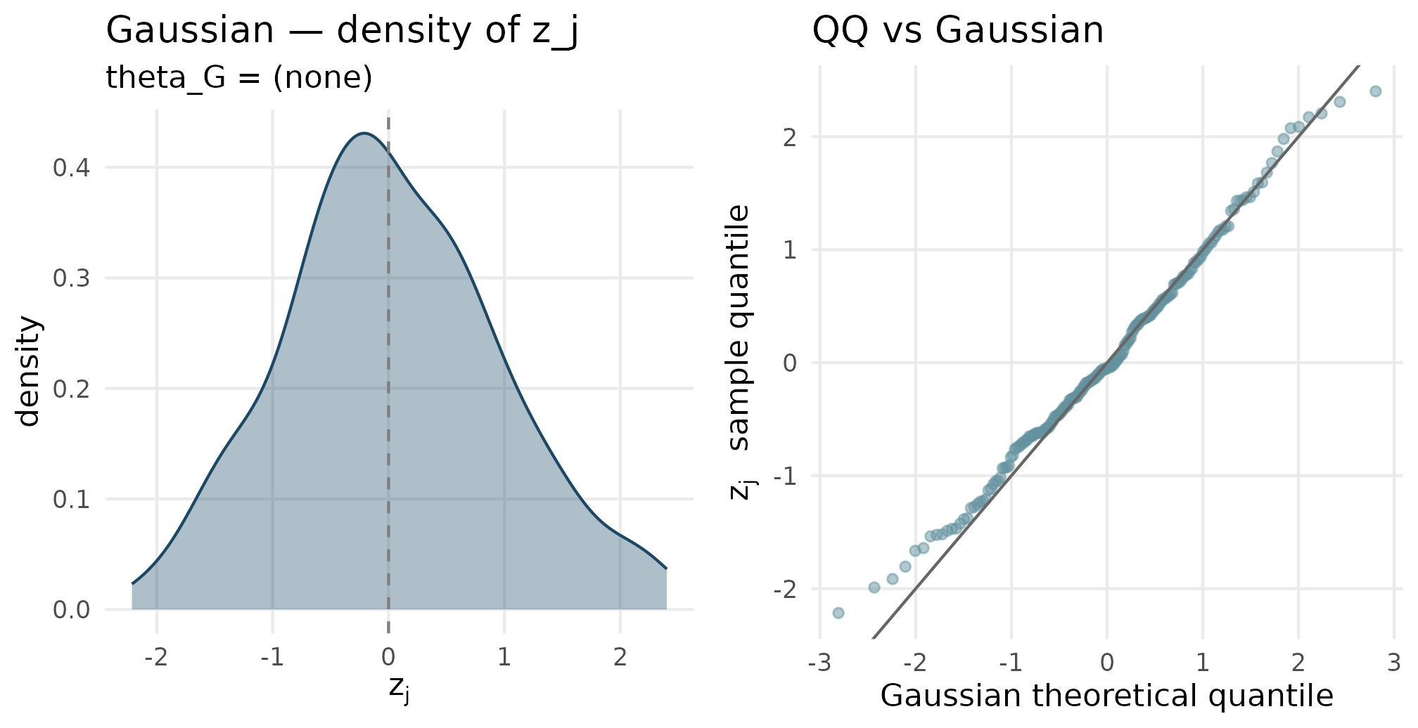

Gaussian density (left) and QQ-against-Gaussian (right). The QQ points sit on the y = x reference line, confirming the realized residuals are Gaussian within sampling fluctuation at J = 200.

6.2 Student-t

plot_density_qq(out_studentt$z_j, "Student-t", "theta_G = list(nu = 5)")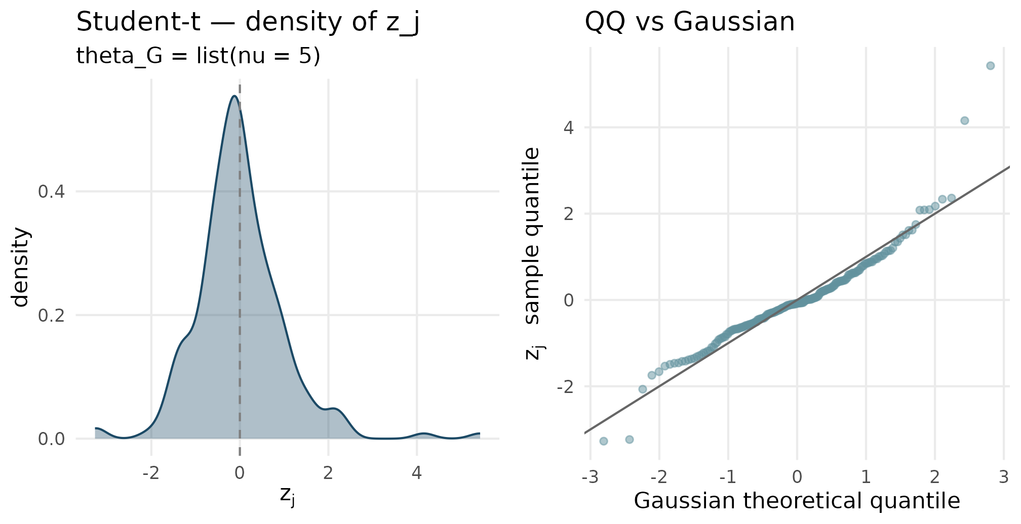

Student-t (nu = 5) density and QQ. Tails of the QQ plot bow away from the y = x line at both ends — the heavy-tail signature relative to Gaussian, the canonical reason to reach for this shape.

6.3 Skew-Normal

plot_density_qq(out_skewn$z_j, "Skew-normal", "theta_G = list(slant = 3)")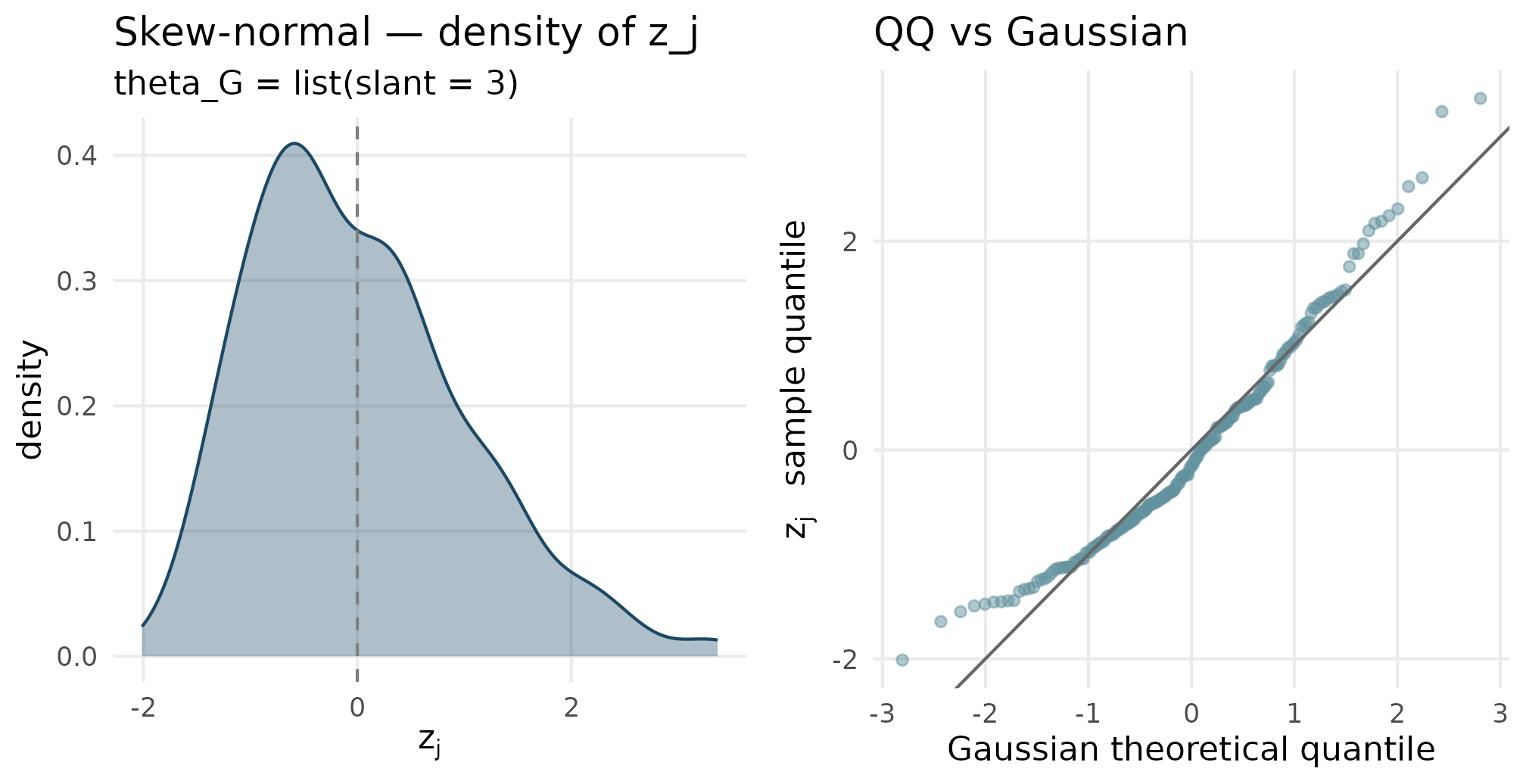

Skew-normal (slant = 3) density and QQ. The density is right-skewed; the upper tail of the QQ plot sits above y = x while the lower tail sits on or above it — the asymmetric signature.

6.4 ALD

plot_density_qq(out_ald$z_j, "ALD", "theta_G = list(rho = 0.3)")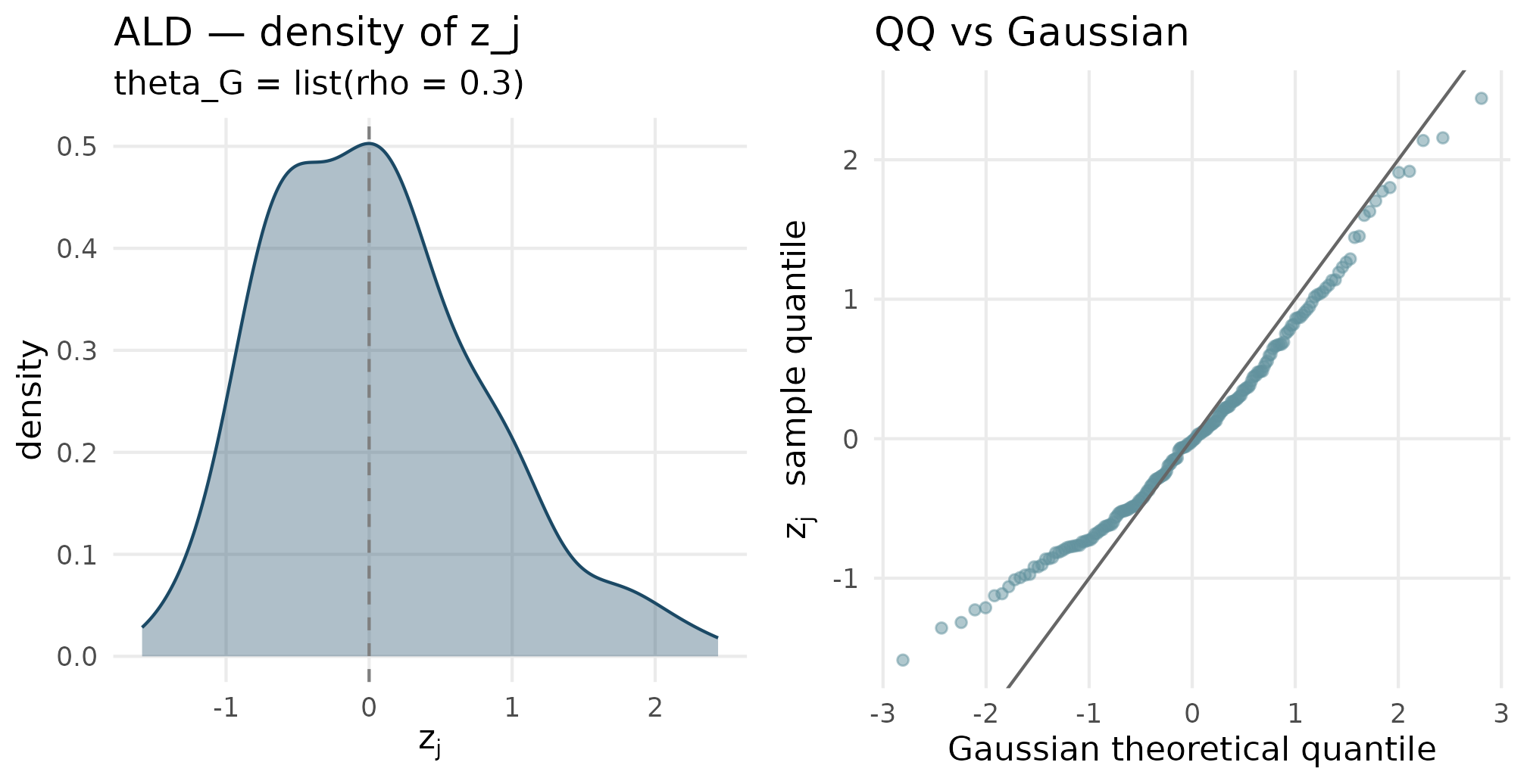

ALD (rho = 0.3) density and QQ. The density has a sharper peak than skew-normal and an exponential tail — the QQ plot shows departures at both tails relative to Gaussian, with a noticeable asymmetry.

6.5 Mixture

plot_density_qq(out_mixture$z_j, "Mixture", "delta = 5, eps = 0.3, ups = 2")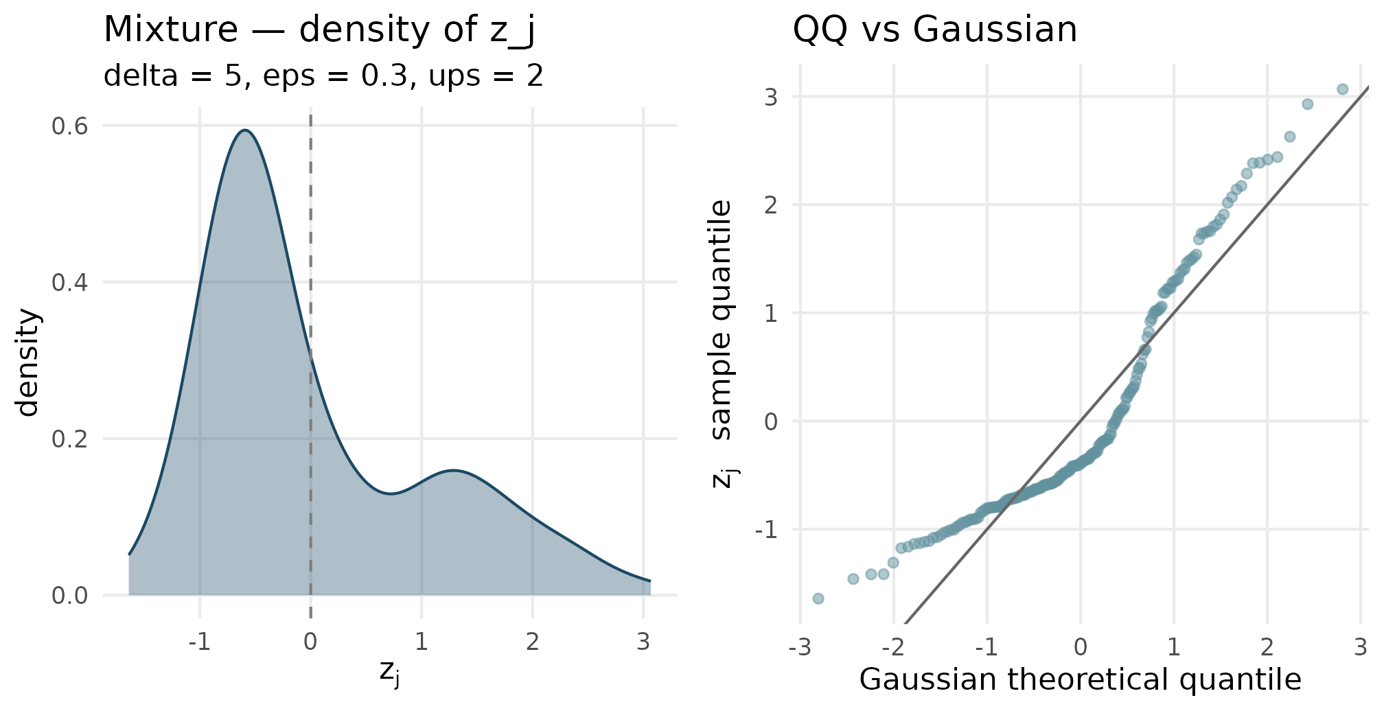

Two-component mixture (delta = 5, eps = 0.3, ups = 2) density and QQ. The density is bimodal — two peaks separated by delta and weighted by eps. The QQ plot has the characteristic step-shape of a bimodal distribution against a unimodal reference.

6.6 Point-mass-plus-slab

plot_density_qq(out_pmslab$z_j, "PointMassSlab", "theta_G = list(pi0 = 0.3)")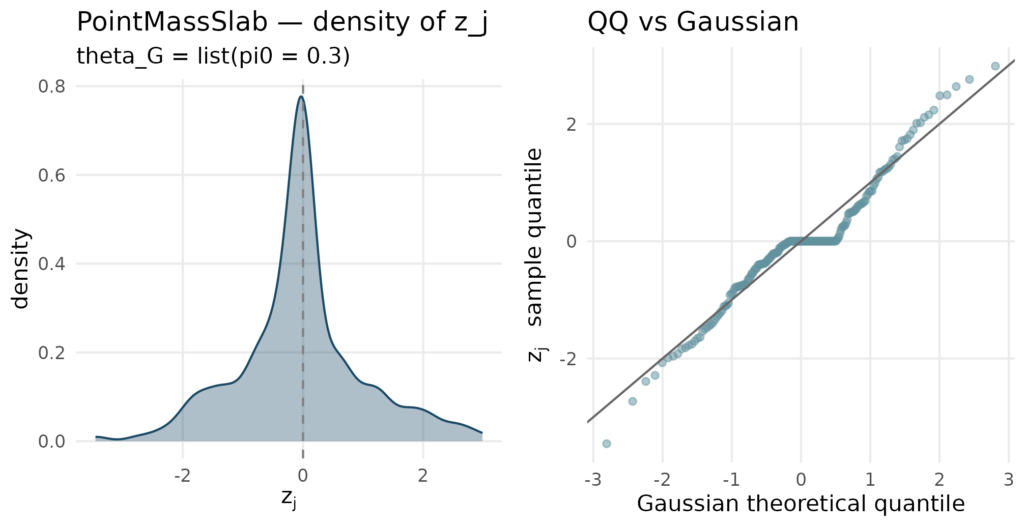

Point-mass-plus-slab (pi0 = 0.3) density and QQ. The density has a visible spike at z = 0 — the point-mass weight — plus a Gaussian-shaped slab. The QQ plot has a flat plateau through the middle quantiles where the spike sits.

6.7 User

plot_density_qq(out_user$z_j, "User (Laplace-shape)", "g_fn = symmetric Laplace, pre-standardized")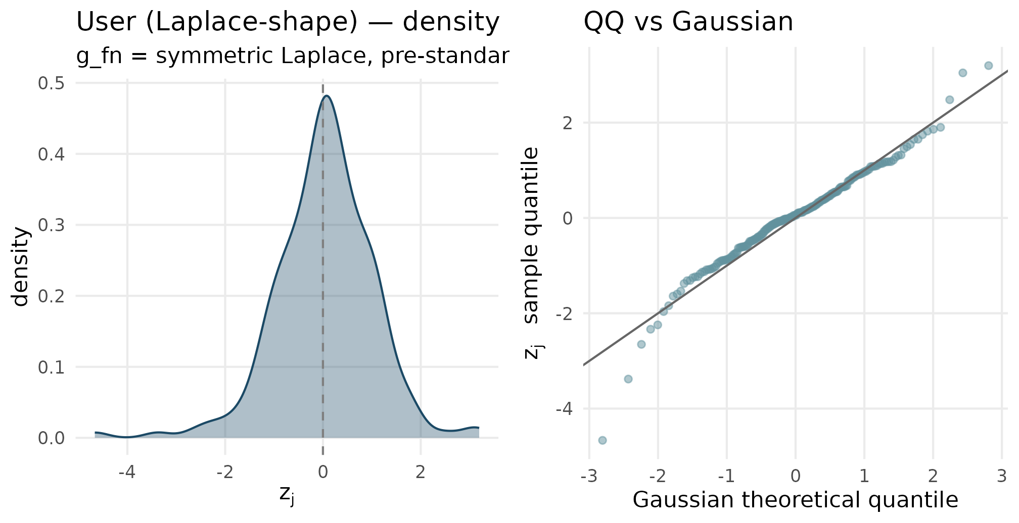

User callback (Laplace-style standardized residuals). The density has a sharper peak than Gaussian and slightly heavier tails — the Laplace signature. The QQ plot bows at both ends similarly to a symmetric heavy-tailed distribution.

6.8 Comparison overlay

A single overlay of all seven density curves on a common axis. Each shape’s signature feature reads off the figure in one glance — the heavy tails of Student-t and User-Laplace, the right skew of SkewN and ALD, the bimodality of Mixture, and the central spike of PointMassSlab.

df_overlay <- dplyr::bind_rows(
  tibble::tibble(z = out_gaussian$z_j, shape = "Gaussian"),
  tibble::tibble(z = out_studentt$z_j, shape = "Student-t (nu = 5)"),
  tibble::tibble(z = out_skewn$z_j,    shape = "SkewN (slant = 3)"),
  tibble::tibble(z = out_ald$z_j,      shape = "ALD (rho = 0.3)"),
  tibble::tibble(z = out_mixture$z_j,  shape = "Mixture (5, 0.3, 2)"),
  tibble::tibble(z = out_pmslab$z_j,   shape = "PMSlab (pi0 = 0.3)"),
  tibble::tibble(z = out_user$z_j,     shape = "User (Laplace)")
)
ggplot(df_overlay, aes(x = z, colour = shape)) +
  geom_density(linewidth = 0.6, alpha = 0.8) +
  geom_vline(xintercept = 0, linetype = "dashed", colour = "grey50") +
  labs(
    x        = expression(z[j]~"  (standardized residual)"),
    y        = "density",
    title    = "Catalog overlay — seven standardized G shapes at J = 200",
    subtitle = "All shapes are unit-variance by construction; tail and skew differences are the only design lever.",
    colour   = NULL
  ) +
  theme_minimal(base_size = 11) +
  theme(panel.grid.minor = element_blank(),
        legend.position = "bottom")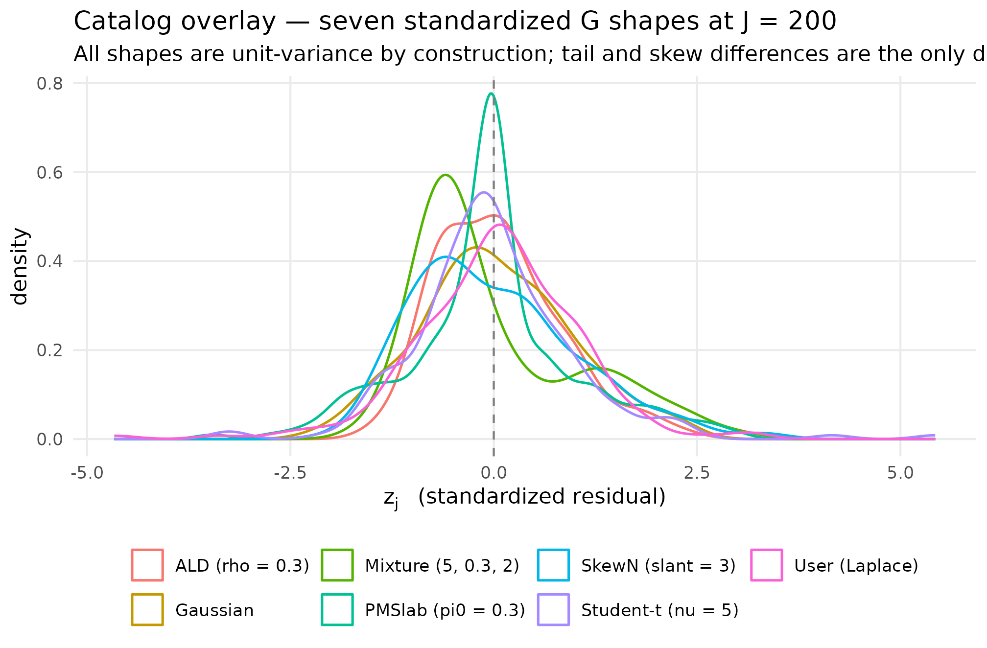

Density overlay of seven shapes at J = 200. Read off: Gaussian is the symmetric reference; Student-t has heavier tails; SkewN has a longer right tail; ALD is sharper-peaked and right-skewed; Mixture is bimodal; PointMassSlab has a central spike at z = 0; User-Laplace is sharper-peaked than Gaussian. The DPM stub is not plotted.

7. Where to next

• M1: The two-stage DGP — the formal specification of the four generative layers; this vignette operationalizes Layer 1’s $G$-shape choice.
• M3: Margin and SE models — the Stage-2 precision marginal; once $z_j$ is fixed, the cross-site spread of $\widehat{se}_j^{\,2}$ is the next design choice.
• M5: Custom G distributions — the long-form treatment of the User callback path, including the audit machinery for Convention A and the recipe for bridging external-distribution samples into the package.
• A2: Choosing a preset — the applied view of how shape choice cascades into the diagnostic readout.
• A8: Cookbook — short walkthroughs that mix shape choice with the rest of the design surface.

References

The factorization $\tau_j = \tau + \sigma_\tau z_j$ with unit-variance standardized residual is the convention adopted in Lee et al. (2025); the empirical-Bayes context is collected in Walters (2024). The skew-normal parameterization is from Azzalini (1985), and the asymmetric Laplace parameterization is from Yu & Zhang (2005). The simulation-design defaults underlying the catalog match the JEBS-paper preset (Lee et al., 2025) and the applied calibration benchmarks (Weiss et al., 2017).

Acknowledgments

This research was supported by the Institute of Education Sciences, U.S. Department of Education, through Grant R305D240078 to the University of Alabama. The opinions expressed are those of the authors and do not represent views of the Institute or the U.S. Department of Education.

Session info

#> R version 4.6.0 (2026-04-24)
#> Platform: x86_64-pc-linux-gnu
#> Running under: Ubuntu 24.04.4 LTS
#> 
#> Matrix products: default
#> BLAS:   /usr/lib/x86_64-linux-gnu/openblas-pthread/libblas.so.3 
#> LAPACK: /usr/lib/x86_64-linux-gnu/openblas-pthread/libopenblasp-r0.3.26.so;  LAPACK version 3.12.0
#> 
#> locale:
#>  [1] LC_CTYPE=C.UTF-8       LC_NUMERIC=C           LC_TIME=C.UTF-8       
#>  [4] LC_COLLATE=C.UTF-8     LC_MONETARY=C.UTF-8    LC_MESSAGES=C.UTF-8   
#>  [7] LC_PAPER=C.UTF-8       LC_NAME=C              LC_ADDRESS=C          
#> [10] LC_TELEPHONE=C         LC_MEASUREMENT=C.UTF-8 LC_IDENTIFICATION=C   
#> 
#> time zone: UTC
#> tzcode source: system (glibc)
#> 
#> attached base packages:
#> [1] stats     graphics  grDevices utils     datasets  methods   base     
#> 
#> other attached packages:
#> [1] ggplot2_4.0.3      multisiteDGP_0.1.1
#> 
#> loaded via a namespace (and not attached):
#>  [1] gtable_0.3.6         jsonlite_2.0.0       dplyr_1.2.1         
#>  [4] compiler_4.6.0       tidyselect_1.2.1     parallel_4.6.0      
#>  [7] gridExtra_2.3        jquerylib_0.1.4      systemfonts_1.3.2   
#> [10] scales_1.4.0         textshaping_1.0.5    yaml_2.3.12         
#> [13] fastmap_1.2.0        R6_2.6.1             labeling_0.4.3      
#> [16] generics_0.1.4       knitr_1.51           tibble_3.3.1        
#> [19] desc_1.4.3           bslib_0.10.0         pillar_1.11.1       
#> [22] RColorBrewer_1.1-3   sn_2.1.3             rlang_1.2.0         
#> [25] utf8_1.2.6           cachem_1.1.0         xfun_0.57           
#> [28] fs_2.1.0             sass_0.4.10          S7_0.2.2            
#> [31] cli_3.6.6            pkgdown_2.2.0        withr_3.0.2         
#> [34] magrittr_2.0.5       digest_0.6.39        grid_4.6.0          
#> [37] lifecycle_1.0.5      vctrs_0.7.3          mnormt_2.1.2        
#> [40] evaluate_1.0.5       glue_1.8.1           numDeriv_2016.8-1.1 
#> [43] farver_2.1.2         ragg_1.5.2           stats4_4.6.0        
#> [46] LaplacesDemon_16.1.8 rmarkdown_2.31       tools_4.6.0         
#> [49] pkgconfig_2.0.3      htmltools_0.5.9

Azzalini, A. (1985). A class of distributions which includes the normal ones. Scandinavian Journal of Statistics, 12(2), 171–178.

Lee, J., Che, J., Rabe-Hesketh, S., Feller, A., & Miratrix, L. (2025). Improving the estimation of site-specific effects and their distribution in multisite trials. Journal of Educational and Behavioral Statistics, 50(5), 731–764. https://doi.org/10.3102/10769986241254286

Walters, C. (2024). Empirical bayes methods in labor economics. In Handbook of labor economics (Vol. 5, pp. 183–260). Elsevier. https://doi.org/10.1016/bs.heslab.2024.11.001

Weiss, M. J., Bloom, H. S., Verbitsky-Savitz, N., Gupta, H., Vigil, A. E., & Cullinan, D. N. (2017). How much do the effects of education and training programs vary across sites? Evidence from past multisite randomized trials. Journal of Research on Educational Effectiveness, 10(4), 843–876. https://doi.org/10.1080/19345747.2017.1300719

Yu, K., & Zhang, J. (2005). A three-parameter asymmetric laplace distribution and its extension. Communications in Statistics — Theory and Methods, 34(9-10), 1867–1879. https://doi.org/10.1080/03610920500199018