M1 · The two-stage DGP — formal specification

JoonHo Lee

2026-05-10

Abstract

For methodologists and reviewers who need the exact specification behind every multisiteDGP call. This vignette derives the joint distribution the package generates from first principles, factors it into the four generative layers, lists twelve testable invariants that pin the implementation to the specification, and maps every symbol used in the package onto the notation of the JEBS paper. You leave with a one-page commutative diagram, a kappa-rate identity check on real simulated output, and a citation-ready notation table.

1. What an analyst sees, what a design encodes

For a multisite trial across $j = 1, \ldots, J$ sites, an analyst who opens a published table sees a tuple per site:

$$\mathcal{D}_j \;=\; \bigl(\hat\tau_j, \;\widehat{se}_j, \;n_j, \;\mathbf{x}_j\bigr).$$

tau_j_hat is the site’s estimated treatment effect, se_j is its sampling standard error, n_j is the within-site sample size, and $\mathbf{x}_j$ collects optional site-level covariates. The covariate vector is genuinely optional: multisiteDGP’s default formula = NULL omits it.

What the analyst does not see — but needs in order to interpret $\hat\tau_j$ — is the latent site effect $\tau_j$ itself: the value $\hat\tau_j$ is estimating. The sampling story says $\hat\tau_j$ varies around $\tau_j$ with magnitude $\widehat{se}_j$. The cross-site story says the $\tau_j$’s vary around a grand mean $\tau$ with cross-site standard deviation $\sigma_\tau$. The package generates both stories simultaneously, and the rest of this vignette specifies exactly how.

Concretely, a multisiteDGP simulation tibble has the seven canonical columns shown below — every Phase 7 vignette uses the same names.

dat_preview <- sim_multisite(preset_jebs_paper(), seed = 1L)
head(tibble::as_tibble(dat_preview)[, c(
  "site_index", "z_j", "tau_j", "tau_j_hat", "se_j", "se2_j", "n_j"
)], 4)
#> # A tibble: 4 × 7
#>   site_index    z_j  tau_j tau_j_hat  se_j  se2_j   n_j
#>        <int>  <dbl>  <dbl>     <dbl> <dbl>  <dbl> <int>
#> 1          1 -0.582 -0.116     0.652 0.426 0.182     22
#> 2          2 -0.619 -0.124    -0.315 0.577 0.333     12
#> 3          3 -1.11  -0.222    -0.633 0.256 0.0656    61
#> 4          4  1.36   0.273     0.357 0.426 0.182     22

The standardized residual z_j and the latent effect tau_j are the two latent quantities the design generates; tau_j_hat, se_j, se2_j, and n_j are the four observable quantities. The specification’s job is to make every conditional and marginal in the seven-column joint precise.

The data-generating process must therefore specify the full joint

$$p\bigl(\hat\tau_j, \widehat{se}_j^{\,2}, n_j, \tau_j \mid \mathbf{x}_j, \boldsymbol\theta\bigr),$$

so that a downstream user can answer at least these five questions [blueprint Ch. 4 §1]:

1. What population does $\hat\tau_j$ inform about? — needs $p(\tau_j)$ with a defined mean and variance.
2. How does precision vary across sites? — needs $p(\widehat{se}_j^{\,2} \mid n_j)$ together with $p(n_j)$.
3. What is the sampling distribution of $\hat\tau_j$ given a site’s true effect and reported precision? — needs $p(\hat\tau_j \mid \tau_j, \widehat{se}_j^{\,2})$.
4. Do covariates explain part of the latent effect? — needs $p(\tau_j \mid \mathbf{x}_j, \cdot)$.
5. Is precision systematically related to the latent effect? — needs the joint structure of $(\tau_j, \widehat{se}_j^{\,2})$.

The four-layer factorization in Section 4 is one natural way to answer all five questions in a single object. Stages 1 and 2 in the next two sections are the conceptual grouping that motivates that factorization.

2. Stage 1 — the sampling distribution

Conditional on the latent site effect $\tau_j$ and on the reported sampling variance $\widehat{se}_j^{\,2}$, the observed estimate is generated as a Gaussian draw:

$$\hat\tau_j \mid \tau_j, \widehat{se}_j^{\,2} \;\sim\; \mathcal{N}\bigl(\tau_j, \;\widehat{se}_j^{\,2}\bigr). \tag{Stage 1}$$

Two points fix the convention. First, the second argument of $\mathcal{N}(\mu, \sigma^2)$ in this package is the variance, never the standard deviation; every formula in this vignette obeys that convention. Second, the Gaussian form is justified by within-site randomization plus a central-limit argument on the difference-in-means estimator $\hat\tau_j = \bar Y_{j,1} - \bar Y_{j,0}$ when the per-arm sample sizes are moderate and the outcome has a finite fourth moment (blueprint Ch. 4 §2.1). The package treats $\widehat{se}_j^{\,2}$ as known (no measurement-error layer on top of it) — this matches the standard meta-analytic convention in which reported standard errors are plugged in (Walters, 2024).

The implementation of this stage lives in gen_observations(), which is the Layer 4 generator in the package’s four-layer factorization. Section 4.4 below makes that connection explicit.

The unbiasedness implied by Stage 1 is the package’s testable invariant T1 (Section 7).

2.1 Stage 1 as a picture

A small simulation makes the conditional concrete. Below, 30 sites are drawn from a Gaussian-shape design with $\sigma_\tau = 0.25$, then the observed estimates $\hat\tau_j$ are overlaid on the latent effects $\tau_j$ on the same axis. The vertical bars give the $\pm 1.96 \cdot \widehat{se}_j$ Gaussian envelope from the Stage-1 conditional.

set.seed(1L)
design_M1 <- multisitedgp_design(
  J            = 30L,
  sigma_tau    = 0.25,
  true_dist    = "Gaussian",
  nj_mean      = 80,
  cv           = 0.5,
  nj_min       = 5,
  p            = 0.5,
  R2           = 0,
  var_outcome  = 1,
  dependence   = "none"
)
dat_M1 <- sim_multisite(design_M1, seed = 1L)
dat_M1
#> # A multisitedgp_data: 30 sites, paradigm = "site_size"
#> # Realized vs intended:
#> #   I: realized=0.519 (no target)
#> #   R: realized=5.560 (no target)
#> #   sigma_tau: target=0.250, realized=0.231, WARN
#> #   rho_S: target=0.000, realized=0.178, PASS
#> #   rho_S_marg: realized=0.178 (no target)
#> #   Feasibility: WARN (n_eff=15.556)
#> # A tibble: 30 × 7
#>   site_index    z_j   tau_j tau_j_hat  se_j  se2_j   n_j
#>        <int>  <dbl>   <dbl>     <dbl> <dbl>  <dbl> <int>
#> 1          1 -0.626 -0.157     0.680  0.348 0.121     33
#> 2          2  0.184  0.0459    0.0379 0.203 0.0412    97
#> 3          3 -0.836 -0.209    -0.0517 0.228 0.0519    77
#> 4          4  1.60   0.399     0.405  0.210 0.0440    91
#> 5          5  0.330  0.0824   -0.111  0.260 0.0678    59
#> 6          6 -0.820 -0.205    -0.168  0.199 0.0396   101
#> # ℹ 24 more rows
#> # Use summary(df) for the full diagnostic report.

The print method’s diagnostic block confirms the realized between-site SD landed near the target 0.25, and that the sampling-variance product $\widehat{se}_j^{\,2} \cdot n_j$ is constant across sites (this is the defining identity of the site-size-driven path — see Section 5.2).

df_stage1 <- tibble::tibble(
  site = seq_len(nrow(dat_M1)),
  tau_j     = dat_M1$tau_j,
  tau_hat_j = dat_M1$tau_j_hat,
  se_j      = dat_M1$se_j
)
df_stage1 <- df_stage1[order(df_stage1$tau_j), ]
df_stage1$rank <- seq_len(nrow(df_stage1))

ggplot(df_stage1, aes(y = rank)) +
  geom_segment(aes(x    = tau_hat_j - 1.96 * se_j,
                   xend = tau_hat_j + 1.96 * se_j,
                   yend = rank),
               colour = "grey70", linewidth = 0.4) +
  geom_point(aes(x = tau_j),     shape = 1, size = 2, colour = "black") +
  geom_point(aes(x = tau_hat_j), shape = 16, size = 1.6, colour = "#1B4965") +
  geom_vline(xintercept = 0, linetype = "dashed", colour = "grey50") +
  scale_y_continuous(breaks = NULL) +
  labs(
    x        = expression(tau[j]~"  /  "~hat(tau)[j]),
    y        = "Sites (sorted by tau_j)",
    title    = "Stage 1 — sampling envelope around latent effect",
    subtitle = "Open = tau_j (latent) · Filled = tau_j_hat (observed) · Bar = +/- 1.96 * se_j"
  ) +
  theme_minimal(base_size = 11) +
  theme(panel.grid.minor = element_blank())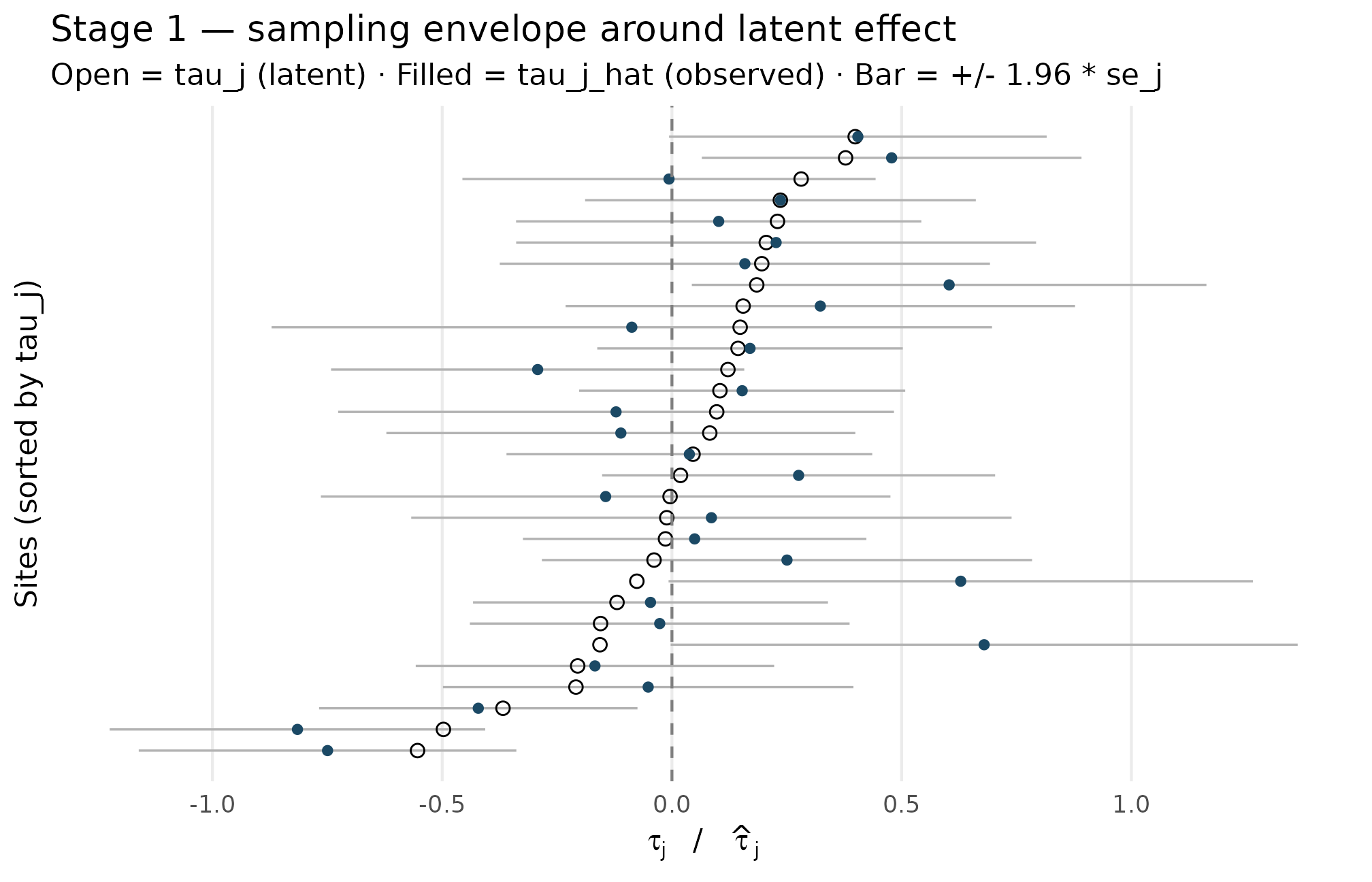

Stage 1 — observed estimates (filled dots) sit around their latent effects (open circles), with sampling envelopes scaled by site-specific se_j. Vertical spread of bar lengths reflects the precision heterogeneity from variation in n_j (range 25 to 139); the overlap between observed and latent values shrinks for the largest sites (narrowest bars). Sampling error is centered on tau_j, confirming the unbiasedness contract of T1.

Three observations to read off the figure. First, the filled dots scatter symmetrically around the open circles — consistent with $E[\hat\tau_j \mid \tau_j] = \tau_j$ (T1). Second, bar widths vary substantially across sites — this is precision heterogeneity, set in Stage 2 by the site-size module (Section 4.2). Third, the bar widths are not correlated with vertical position in the figure — consistent with the design’s dependence = "none" choice (T7).

3. Stage 2 — the generative model on $(\tau_j, \widehat{se}_j^{\,2})$

Stage 1 takes $\tau_j$ and $\widehat{se}_j^{\,2}$ as inputs. Stage 2 is where they come from. The Stage-2 joint factors as a marginal on the latent effect, a precision module, and an explicit dependence coupling:

$$p\bigl(\tau_j, \widehat{se}_j^{\,2} \mid \mathbf{x}_j, \boldsymbol\theta\bigr) = \underbrace{p\bigl(\tau_j \mid \mathbf{x}_j, \boldsymbol\theta_G\bigr)}_{\text{latent effect}} \;\cdot\; \underbrace{p\bigl(\widehat{se}_j^{\,2} \mid n_j, \kappa\bigr) \cdot p\bigl(n_j \mid \bar n_j, \mathrm{CV}, n_{j,\min}\bigr)}_{\text{precision via site size}} \;\cdot\; \underbrace{c\bigl(\tau_j, \widehat{se}_j^{\,2}\bigr)}_{\text{coupling}}.$$

The default — and what Stage-1 unbiasedness reduces the package to in the absence of any dependence injection — is $c(\cdot, \cdot) \equiv 1$, i.e. $\tau_j$ and $\widehat{se}_j^{\,2}$ are independent given the design parameters [blueprint Ch. 4 §2.5]. The package allows that independence to be broken via a post-hoc rearrangement step (Section 5); this is the package’s precision dependence feature, kept optional and off by default so that the JEBS-paper specification is recovered exactly when the user does not opt in.

The next section makes the four pieces of this Stage-2 joint into four named layers and gives each one its conditional distribution.

4. The four generative layers

The full joint, written across all of Stages 1 and 2, factors into four layers in a fixed order: latent effects → site-size margins → precision dependence → observation draws. Each layer corresponds to one named generator family in the package, and one section of this vignette below.

$$\underbrace{p\bigl(\tau_j \mid \tau, \sigma_\tau, \boldsymbol\theta_G, \mathbf{x}_j, \boldsymbol\beta\bigr)}_{\text{Layer 1 (latent effects)}} \;\cdot\; \underbrace{p\bigl(n_j \mid \bar n_j, \mathrm{CV}, n_{j,\min}\bigr) \cdot p\bigl(\widehat{se}_j^{\,2} \mid n_j, \kappa\bigr)}_{\text{Layer 2 (site-size margins)}} \;\cdot\; \underbrace{c\bigl(\tau_j, \widehat{se}_j^{\,2}\bigr)}_{\text{Layer 3 (precision dependence)}} \;\cdot\; \underbrace{p\bigl(\hat\tau_j \mid \tau_j, \widehat{se}_j^{\,2}\bigr)}_{\text{Layer 4 (observation draws)}}.$$

The order is operational: Layer 1 fills z_j and tau_j, Layer 2 fills n_j and se2_j (and therefore se_j), Layer 3 (when active) permutes the precisions to induce a target rank correlation with the effects, and Layer 4 fills tau_j_hat. The four layers are also the four S3 generators gen_effects(), gen_site_sizes(), align_rank_corr() (and its copula and hybrid siblings), and gen_observations().

4.1 Layer 1 — latent effects

Site labels carry no information by design — they are interchangeable. de Finetti’s exchangeability theorem then implies that the latent effects are conditionally i.i.d. from some mixing distribution $G$:

$$\tau_j \mid \tau, \sigma_\tau, \boldsymbol\theta_G \;\stackrel{\text{i.i.d.}}{\sim}\; G\bigl(\,\cdot\,;\, \tau, \sigma_\tau, \boldsymbol\theta_G\bigr), \qquad E[\tau_j] = \tau, \;\; \mathrm{Var}(\tau_j) = \sigma_\tau^{\,2}.$$

This corresponds to JEBS Equation (2) when $G$ is taken to be Gaussian (Lee et al., 2025). The package implements eight choices for $G$ — Gaussian, two-component mixture, asymmetric Laplace (Yu & Zhang, 2005), Student-t, skew-normal (Azzalini, 1985), point-mass-plus-slab, a user-supplied callback, and a Dirichlet process mixture stub. The catalog and standardization details live in M2: G-distribution catalog; for the purposes of M1, the only contract that matters is that every member of the catalog has mean $\tau$ and variance $\sigma_\tau^{\,2}$ on the output scale.

The package factors $\tau_j$ as a location plus a scaled standardized residual:

$$\tau_j \;=\; \tau + \sigma_\tau \, z_j, \qquad z_j \sim G_0, \;\; E[z_j] = 0, \;\; \mathrm{Var}(z_j) = 1,$$

where $G_0$ is the standardized version of the chosen $G$ shape. The column z_j in the simulation tibble is exactly this standardized residual. Var $z_j = 1$ is the package’s testable invariant T2 (Section 7), and writing the latent effect this way is what makes the covariate-augmented form

$$\tau_j \;=\; \tau + \mathbf{x}_j^{\!\top}\boldsymbol\beta + \sigma_\tau\, z_j$$

a transparent extension rather than a reparameterization. Under covariates, $\sigma_\tau$ is the residual between-site SD — the marginal SD also picks up $\mathrm{Var}(\mathbf{x}_j^{\!\top}\boldsymbol\beta)$. This is why print.multisitedgp_data() shows two $\sigma_\tau$ values when covariates are active. The covariate-augmented case is the subject of A4: Covariates and precision dependence; the covariate-off identity $\sigma_\tau^{\text{resid}} = \sigma_\tau^{\text{marg}}$ is the package’s testable invariant T6.

4.2 Layer 2 — site-size margins

Two pieces. First, site sample sizes $n_j$ are drawn from a truncated Gamma distribution moment-matched to the user-supplied mean $\bar n_j$ and coefficient of variation $\mathrm{CV}$, with a hard lower bound at $n_{j,\min}$ [blueprint Ch. 4 §2.4]:

$$n_j \;\stackrel{\text{i.i.d.}}{\sim}\; \mathrm{TruncGamma}\bigl(\bar n_j,\, \mathrm{CV};\; n_{j,\min}\bigr).$$

The default $n_{j,\min} = 5$ is enforced as the package’s testable invariant T10 (Section 7); the truncation is the reason no multisite simulation ever produces an $n_j$ smaller than 5 by default. The truncated-Gamma form is the modern Engine A2; the legacy JEBS-appendix Engine A1 uses a censor-and-round form instead, and the two engines exist precisely so that the JEBS appendix is reproducible bit-for-bit (T1a) without giving up modern moment-matching (T1b). See M3: Margin and SE models for the engine contracts.

Second, conditional on $n_j$, the per-site sampling variance is set deterministically:

$$\widehat{se}_j^{\,2} \;=\; \frac{\kappa}{n_j},$$

with the proportionality constant $\kappa$ derived from a balanced two-arm randomization with allocation share $p$, residual outcome variance $s_Y^2$, and covariate-explained share $R^2$:

$$\kappa \;=\; \left(\frac{1}{p} + \frac{1}{1-p}\right)(1 - R^2)\, s_Y^2.$$

At the package defaults $p = 0.5$, $R^2 = 0$, $s_Y^2 = 1$, this collapses to $\kappa = 4$. The deterministic form is what makes the identity $\widehat{se}_j^{\,2} \cdot n_j = \kappa$ hold for every site in every simulation under the site-size-driven path — this is the package’s testable invariant T3 (Section 7) and the defining contract of the path itself. A minute of code makes it visible:

range(dat_M1$se2_j * dat_M1$n_j)
#> [1] 4 4
unique(round(dat_M1$se2_j * dat_M1$n_j, 8))
#> [1] 4
compute_kappa(p = 0.5, R2 = 0, var_outcome = 1)
#> [1] 4

The first line shows the kappa-rate product is constant. The third line confirms the closed form returns 4.

The alternative direct-precision path (gen_se_direct()) discards the deterministic kappa identity in exchange for direct control of the informativeness scalar $I$ and the precision heterogeneity ratio $R$; that path is the subject of M3 §3 and is outside the scope of this vignette except as part of the JEBS notation table in Section 6.

4.3 Layer 3 — precision dependence

By default, $\tau_j$ and $\widehat{se}_j^{\,2}$ are independent because they are generated from independent random draws. When a user asks for a non-zero target Spearman or Pearson correlation, the package performs a post-hoc rearrangement of the precisions so that their multiset is preserved exactly while their pairing with effects matches the target.

Three coupling functions are exposed: align_rank_corr() (rank permutation), align_copula_corr() (Gaussian copula re-pairing), and align_hybrid_corr() (copula initialization plus rank refinement). The methodological contrast across the three lives in M4: Precision dependence theory.

The contracts that matter for M1 are:

• When dependence = "none", the coupling reduces to the identity permutation (T7). No rearrangement, no change to either marginal.
• The marginal of $\tau_j$ is preserved exactly (its mean, variance, and shape are not touched).
• The multiset of $\widehat{se}_j^{\,2}$ is preserved exactly (its realized values are not touched, only their pairing with sites is).
• The realized informativeness $I$ is preserved exactly across any active rearrangement.

The reason the package generates first and rearranges second — rather than building dependence into a joint distribution upfront — is to keep the user’s specification of the marginals from drifting. T7 is the testable contract that the rearrangement is genuinely identity when the user opts out.

4.4 Layer 4 — observation draws

Layer 4 is the implementation of Stage 1 from Section 2: given the latent effects produced by Layer 1 and the sampling variances produced by Layer 2 (possibly rearranged in Layer 3), draw

$$\hat\tau_j \;\sim\; \mathcal{N}\bigl(\tau_j, \;\widehat{se}_j^{\,2}\bigr), \qquad j = 1, \ldots, J,$$

independently across $j$. The implementation is gen_observations(); the column tau_j_hat in the simulation tibble is its output.

Independence of the per-site $\hat\tau_j$ draws (conditional on Layer 1–3 outputs) is part of the same blueprint Ch. 4 §2.5 default. It is not a separate testable invariant — it is the defining form of the observation generator. T1 in Section 7 covers the unbiasedness contract; the conditional independence of the draws is structural.

4.5 The Stage-2 joint as a picture

The default joint $p(\tau_j, \widehat{se}_j^{\,2})$ — independent marginals, no dependence coupling — looks like this. The two density panels show the marginal of each axis, and the central scatter shows the realized pairs.

set.seed(2L)
design_marg <- multisitedgp_design(
  J            = 200L,
  sigma_tau    = 0.25,
  true_dist    = "Gaussian",
  nj_mean      = 60,
  cv           = 0.5,
  nj_min       = 5,
  p            = 0.5,
  R2           = 0,
  var_outcome  = 1,
  dependence   = "none"
)
dat_marg <- sim_multisite(design_marg, seed = 2L)

sd_tau    <- round(sd(dat_marg$tau_j), 4)
gm_se2    <- round(exp(mean(log(dat_marg$se2_j))), 4)
range_se2 <- range(dat_marg$se2_j)
sd_tau; gm_se2; range_se2
#> [1] 0.2685
#> [1] 0.0791
#> [1] 0.01960784 0.50000000

df_marg <- tibble::tibble(
  tau_j  = dat_marg$tau_j,
  se2_j  = dat_marg$se2_j
)

p_center <- ggplot(df_marg, aes(x = tau_j, y = se2_j)) +
  geom_point(alpha = 0.45, size = 1.6, colour = "#1B4965") +
  geom_vline(xintercept = 0, linetype = "dashed", colour = "grey50") +
  labs(
    x = expression(tau[j]~"  (latent effect)"),
    y = expression(widehat(se)[j]^{2}~"  (sampling variance)")
  ) +
  theme_minimal(base_size = 11) +
  theme(panel.grid.minor = element_blank())

p_top <- ggplot(df_marg, aes(x = tau_j)) +
  geom_density(fill = "#1B4965", alpha = 0.35, colour = "#1B4965") +
  labs(x = NULL, y = "density") +
  theme_minimal(base_size = 9) +
  theme(panel.grid.minor = element_blank(),
        axis.text.x  = element_blank(),
        axis.ticks.x = element_blank())

p_right <- ggplot(df_marg, aes(x = se2_j)) +
  geom_density(fill = "#62929E", alpha = 0.45, colour = "#62929E") +
  coord_flip() +
  labs(x = NULL, y = "density") +
  theme_minimal(base_size = 9) +
  theme(panel.grid.minor = element_blank(),
        axis.text.y  = element_blank(),
        axis.ticks.y = element_blank())

# Compose without depending on patchwork (soft dep).
gridExtra::grid.arrange(
  p_top,                                grid::nullGrob(),
  p_center,                             p_right,
  ncol = 2, widths = c(4, 1), heights = c(1, 4)
)

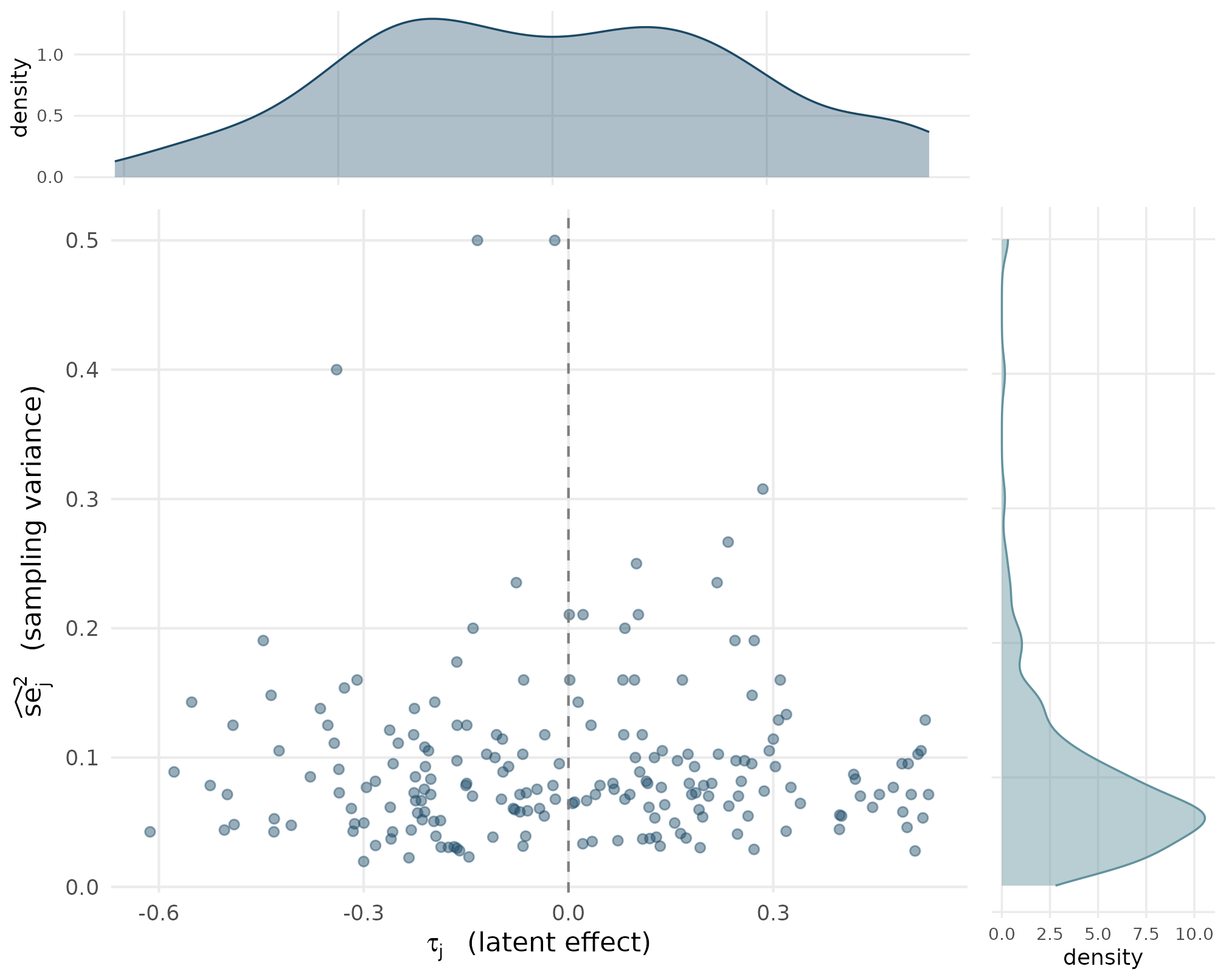
Stage 2 default joint p(tau_j, se_j squared) at J = 200. Top: marginal density of latent effects, centered near 0 with SD near sigma_tau = 0.25 (T2). Right: marginal density of sampling variances, right-skewed because n_j is right-skewed and se squared = kappa over n_j (T3). Center: scatter of realized (tau_j, se squared) pairs is roughly cloud-shaped, with no visible tilt — independence at the sample level, consistent with T7.

Three things to read off the joint:

• The top panel’s density is centered near zero and has spread close to $\sigma_\tau = 0.25$. This is T2 in action: the standardized residual has unit variance, so $\tau_j$’s marginal SD lands at $\sigma_\tau$.
• The right panel’s density is right-skewed. That is the deterministic consequence of $\widehat{se}_j^{\,2} = \kappa / n_j$ (T3) plus the truncated-Gamma marginal on $n_j$: large $n_j$ pile up near the mean, but small $n_j$ pull the SE-squared distribution out to the right.
• The central scatter is roughly cloud-shaped. There is no systematic tilt — the realized rank correlation between $\tau_j$ and $\widehat{se}_j^{\,2}$ is statistically indistinguishable from zero at $J = 200$. This is T7 in action.

5. Default-mode reduction

When every option is at its default value, the package reduces to a short, vanilla two-stage random-effects model. Defaults are true_dist = "Gaussian", formula = NULL, dependence = "none", the site-size-driven path (Paradigm A in the blueprint), and $p = 0.5$, $R^2 = 0$, $s_Y^2 = 1$ giving $\kappa = 4$:

$$\boxed{ \begin{aligned} n_j &\;\stackrel{\text{i.i.d.}}{\sim}\; \mathrm{TruncGamma}(\bar n_j, \mathrm{CV};\, n_{j,\min} = 5),\\ \widehat{se}_j^{\,2} &= 4 / n_j,\\ \tau_j &\;\stackrel{\text{i.i.d.}}{\sim}\; \mathcal{N}(\tau, \sigma_\tau^{\,2}),\\ \hat\tau_j \mid \tau_j, \widehat{se}_j^{\,2} &\;\sim\; \mathcal{N}\bigl(\tau_j, \widehat{se}_j^{\,2}\bigr). \end{aligned}}$$

This is the site-size-driven path’s default form; the JEBS-paper specification is contained inside it as a special case (Lee et al., 2025). Section 6 maps every symbol to JEBS notation, and Section 7 lists the twelve invariants the package carries.

5.1 Two paths through Stage 2

The blueprint distinguishes two ways to set the precision marginal. The site-size-driven path (Paradigm A in the blueprint) is what Section 4.2 derived: a user supplies $\bar n_j$, $\mathrm{CV}$, and $\kappa$; sites sizes $n_j$ are drawn; precisions follow as $\widehat{se}_j^{\,2} = \kappa / n_j$. The direct-precision path (Paradigm B in the blueprint) inverts: a user supplies the informativeness scalar $I$ and the precision heterogeneity ratio $R$, and the precision marginal is reconstructed (log-evenly spaced) to match. The default is the site-size-driven path; the direct-precision path is the subject of M3: Margin and SE models. The notation table in Section 6 covers symbols from both paths.

5.2 Three deviations from the default

Three knobs, each with a default that recovers the JEBS-paper specification, expand the package beyond the JEBS scope:

• Covariate-augmented Stage 2 — passing a formula with data and beta introduces the linear term $\mathbf{x}_j^{\!\top} \boldsymbol\beta$ (Section 4.1). With formula = NULL, the unconditional and covariate-augmented code paths are identical to floating-point precision (T5).
• Precision dependence — setting dependence to rank, copula, or hybrid activates Layer 3’s rearrangement (Section 4.3). With dependence = "none", the rearrangement reduces to identity (T7).
• G-shape choice — setting true_dist to one of the seven non-Gaussian shapes (Section 4.1) selects from M2’s catalog. With true_dist = "Gaussian", the latent effects follow JEBS Equation
  2. exactly.

6. JEBS notation map

This section maps every symbol the package uses onto the notation of the JEBS paper (Lee et al., 2025). The table is split into three parts: equations from the body of the JEBS paper, simulation-design formulas from the JEBS appendix code, and package-only extensions that have no JEBS counterpart.

6.1 JEBS paper body equations

JEBS reference	Symbol / equation	Package mapping	Notes
Stage-1 setup (unnumbered)	$\hat\tau_j \mid \tau_j, \widehat{se}_j^{\,2} \sim \mathcal{N}(\tau_j, \widehat{se}_j^{\,2})$	gen_observations()	Justified by within-site randomization + CLT
Eq. (1)	$\widehat{se}_j^{\,2} = \bigl(\tfrac{1}{p_j} + \tfrac{1}{1-p_j}\bigr) s_j^{\,2} (1 - R^2) / n_j$	compute_kappa() (closed form)	Per-site SE under balanced randomization
Eq. (2)	$\tau_j \mid \tau, \sigma^2 \sim \mathcal{N}(\tau, \sigma^2)$	gen_effects() with true_dist = "Gaussian"	Default G shape; mean $\tau$, variance $\sigma_\tau^{\,2}$
Eq. (3)	Posterior shrinkage estimator	(out of DGP scope)	Estimator side; covered in siteBayes2, not multisiteDGP
Eq. (4)	$I = \sigma^2 / (\sigma^2 + \exp(\overline{\ln \widehat{se}_j^{\,2}}))$	informativeness()	Generative-side diagnostic

6.2 JEBS appendix simulation formulas

Appendix reference	Symbol / construct	Package mapping	Notes
Appendix mixture form	Two-component mixture with parameters $\delta, \varepsilon, \nu$	gen_effects() with true_dist = "Mixture"	Bit-identical with appendix code under Engine A1 (T1a)
Appendix site-size + SE form	$n_j$ Gamma + censor + round; $\widehat{se}_j^{\,2} = \kappa / n_j$	gen_site_sizes() Engine A1	T1a fixture
Appendix observation form	$\hat\tau_j \sim \mathcal{N}(\tau_j, \widehat{se}_j^{\,2})$ + row shuffle	gen_observations() Engine A1 path	Order of RNG calls is itself an invariant (T12)
Appendix default	$p = 0.5$, $R^2 = 0$, $s_Y^2 = 1$ → $\kappa = 4$	multisitedgp_design() defaults	T2/T3 fixture
Appendix G shapes	Gaussian, two-component mixture, asymmetric Laplace	gen_effects() true_dist ∈ {Gaussian, Mixture, ALD}	Three of the package’s eight shapes
Appendix site-size marginal	$n_j \sim \mathrm{TruncGamma}(\bar n_j, \mathrm{CV} \cdot \bar n_j; n_{j,\min} = 5)$	gen_site_sizes() Engine A2	T10 fixture

6.3 Package-only extensions

Feature	Symbol / construct	Package mapping	Notes
Site-level covariates	$\tau_j = \tau + \mathbf{x}_j^{\!\top} \boldsymbol\beta + \sigma_\tau z_j$	gen_effects() with formula, beta, data	Reduces to JEBS Eq. (2) when formula = NULL (T5)
Precision dependence (rank)	Target Spearman $\rho_S$ between $\tau_j$ (or $z_j$) and $\widehat{se}_j^{\,2}$	align_rank_corr()	Identity permutation when dependence = "none" (T7)
Precision dependence (copula)	Target Pearson $\rho_P$ via Gaussian copula	align_copula_corr()	M4 vignette covers selection criteria
Precision dependence (hybrid)	Copula initialization + rank refinement	align_hybrid_corr()	M4 vignette covers when each path is appropriate
Direct-precision path	Inverse design from $(I, R)$ to $\widehat{se}_j^{\,2}$ marginal	gen_se_direct()	M3 vignette covers feasibility region
Five new G shapes	Student-t, skew-normal (Azzalini, 1985), point-mass-plus-slab, user, DPM stub	gen_effects() true_dist ∈ {StudentT, SkewN, PointMassSlab, User, DPM}	Five of the package’s eight shapes; Gaussian default preserves JEBS Eq. (2)

7. Twelve testable invariants

The specification in Sections 1–4 is only as precise as the implementation it pins down. Twelve invariants, each a one-line contract on observable output, form the testable backbone of this correspondence — every one of them lives in tests/testthat/test-jebs-parity.R and surrounding test files in the package source. The numbering follows the blueprint Ch. 4 §7 listing, with T1 split into T1a (Engine A1, bit-identical with the JEBS appendix) and T1b (Engine A2, distributional parity) per the blueprint’s R1.4 fix.

T1a — Engine A1 bit-identical parity (mixture)

Engine A1 (legacy, legacy_jebs_censor_round) under the JEBS appendix’s exact configuration — true_dist = "Mixture" with $(\delta, \varepsilon, \nu) = (5, 0.3, 2)$, $J = 100$, $\bar n_j = 80$, $\mathrm{CV} = 0.5$, $n_{j,\min} = 4$, formula = NULL, dependence = "none" — produces a simulation tibble whose xxhash64 digest matches the digest of the JEBS appendix pipeline output across the seed set $\{42, 1, 2024, 12345\}$. Bit-identical means floating-point byte equality, not distributional similarity.

T1b — Engine A2 distributional parity (Gaussian)

Engine A2 (modern, trunc_gamma_moment) with true_dist = "Gaussian" and the package defaults ($J = 50$, $\sigma_\tau = 0.25$, $\bar n_j = 80$, $\mathrm{CV} = 0.5$, $n_{j,\min} = 5$, $p = 0.5$, $R^2 = 0$, $s_Y^2 = 1$) produces $\tau_j$ samples whose empirical mean is within $2\sigma_\tau / \sqrt{J}$ of $\tau$, whose empirical variance is within $2\sigma_\tau^{\,2} / \sqrt{J}$ of $\sigma_\tau^{\,2}$, and whose KS test against $\mathcal{N}(\tau, \sigma_\tau^{\,2})$ passes at the 0.05 level in at least 95 percent of $M = 1000$ Monte Carlo replications. Distributional parity, not bit-identical.

T2 — kappa is exactly 4 at defaults

At $p = 0.5$, $R^2 = 0$, $s_Y^2 = 1$, the realized $\kappa$ equals 4 exactly (no rounding). This is the bridge from the closed form $\kappa = (1/p + 1/(1-p))(1 - R^2) s_Y^2$ to the package output the user sees. Verified directly:

compute_kappa(p = 0.5, R2 = 0, var_outcome = 1)
#> [1] 4
identical(compute_kappa(p = 0.5, R2 = 0, var_outcome = 1), 4)
#> [1] TRUE

T3 — kappa-rate identity holds for every site

Under the site-size-driven path, $\widehat{se}_j^{\,2} \cdot n_j = \kappa$ for every $j$ to floating-point precision. Equivalently, the within-design variance of $n_j \cdot \widehat{se}_j^{\,2}$ across $j$ is zero. The check on dat_M1 from Section 4.2 is the operational form of this contract.

T4 — Stage-2 independence under dependence = "none"

When dependence = "none", the realized Spearman and Pearson correlations between $\tau_j$ and $\widehat{se}_j^{\,2}$ are statistically indistinguishable from zero. The acceptance band is the empirical 95th percentile of $|\hat\rho_S|$ from 1000 random independent permutations (a permutation envelope) — not the Fisher-z asymptotic critical value, which is a Pearson approximation that is tight but inexact for Spearman. The blueprint corrected an earlier draft on this point; the package follows the permutation form.

T5 — covariate-off equivalence

When formula = NULL (or when the user passes beta = 0), the covariate-augmented code path produces output identical to the unconditional path to floating-point precision ($\epsilon = 10^{-12}$). This is what makes the package’s covariate handling a strict extension rather than a reparameterization.

T6 — residual equals marginal SD when no covariates

When formula = NULL, the print.multisitedgp_data() method reports sigma_tau_resid and sigma_tau_marg as numerically identical, and both equal the input sigma_tau to floating-point precision. With covariates, the marginal SD picks up $\mathrm{Var}(\mathbf{x}_j^{\!\top}\boldsymbol\beta)$ and the two quantities diverge — see A4.

T7 — precision dependence reduces to identity

When dependence = "none", the alignment functions align_rank_corr(), align_copula_corr(), and align_hybrid_corr() all reduce to the identity permutation: input vector equals output vector, exactly. This is the operational form of the “off by default” contract on Layer 3.

T8 — informativeness formula

informativeness() implements JEBS Equation (4) verbatim:

$$I \;=\; \frac{\sigma_\tau^{\,2}}{\sigma_\tau^{\,2} + \exp\bigl(\overline{\ln \widehat{se}_j^{\,2}}\bigr)},$$

where the bar denotes the arithmetic mean over $j = 1, \ldots, J$. Section 6.1 entry for Eq. (4) is the same statement.

T9 — default G shape is Gaussian

When true_dist is omitted, the package defaults to "Gaussian". At $J \in \{50, 200\}$ across $M = 1000$ Monte Carlo replications, the Shapiro-Wilk test against $\mathcal{N}(\tau, \sigma_\tau^{\,2})$ rejects at the 0.01 level a count consistent with the binomial acceptance interval — concretely, the count of $p \le 0.01$ events falls in $[\mathrm{qbinom}(0.025, M, 0.01),\, \mathrm{qbinom}(0.975, M, 0.01)] = [4, 17]$ for $M = 1000$. The acceptance band acknowledges that under a true normal, the Shapiro-Wilk $p$-value is uniform, so the count of small $p$-values is itself a binomial random variable.

T10 — site-size truncation enforces $n_{j,\min}$

At $n_{j,\min} = 5$, no $n_j < 5$ ever appears in the simulation output, and the realized mean $\bar n_j$ is within $\pm 0.5$ percent of the requested mean. The truncation is hard, not soft, in both engines.

T11 — informativeness range matches JEBS over the design grid

Across the JEBS simulation grid — $J \in \{25, 50, 100, 200, 300\}$, $\bar n_j \in \{10, 20, 40, 80, 160\}$, $\mathrm{CV} \in \{0, 0.25, 0.50, 0.75\}$, $\sigma_\tau \in \{0.05, 0.10, 0.15, 0.20, 0.25\}$ giving $5 \times 5 \times 4 \times 5 = 500$ design cells — the realized informativeness values cover the JEBS-reported range $I \in [0.01, 0.71]$ (Lee et al. 2025, p. 13). The full grid is the contract; a default-CV slice is not sufficient.

T12 — Engine A1 RNG sequence is locked

Under Engine A1, the random-number-generator call sequence is exactly: rgamma(J) for site sizes, rnorm(J) for the first noise draw, then the row-shuffle internal sample() call from dplyr::slice_sample(prop = 1), then rnorm(J) for any subsequent noise. No additional RNG calls. Reordering, omitting the slice_sample shuffle, or re-seeding mid-pipeline all violate T12 and break T1a parity simultaneously. Engine A2’s RNG sequence is separate and is the subject of T20 in the blueprint (out of M1 scope).

How the invariants relate to the four layers

A short cross-reference, for orientation:

Invariant	Layer	What it pins
T1, T1a, T1b	Layer 4 (and Engine A1/A2 pipelines end-to-end)	Stage 1 unbiasedness; appendix bit-equivalence; modern distributional parity
T2, T3	Layer 2	$\kappa = 4$ at defaults; deterministic kappa-rate identity
T4, T7	Layer 3	Independence under dependence = "none"; identity permutation contract
T5, T6	Layer 1	Covariate-off equivalence; residual-equals-marginal SD
T8, T11	Cross-layer (diagnostics)	Informativeness formula; informativeness range
T9	Layer 1	Default G shape is Gaussian
T10	Layer 2	Site-size truncation
T12	Engine A1	RNG call order locked to JEBS appendix

Forward pointers — T13–T20 in companion vignettes

T1–T12 above are the invariants that fit naturally inside the two-stage DGP specification this vignette covers. The blueprint’s full T-numbered list extends further; the remaining invariants live with the layer they constrain:

• T13–T17 — per-shape unit-variance standardization — checks that ALD, Mixture, Student-$t$, skew-normal, and point-mass-slab generators all return $\mathrm{Var}(z_j) = 1$ at the package’s closed-form rescalers. Operationalized in M2: G-distribution catalog and standardization §4 (sanity checks) and the package’s $J = 10^6$ test suite.
• T18–T19 — covariate decomposition + Spearman tie handling — identifiability of the residual / marginal split when covariates enter Layer 1, and the rank-correlation behavior at tied precision values. Operationalized in A4: Covariates and precision dependence for the residual-vs-marginal demonstration and in M4: Precision dependence theory §3.2 for the rank ties.
• T20 — Engine A2 reproducibility — the modern-engine RNG-call sequence (the analogue of T12 for Engine A2) and its hash determinism across reruns. Operationalized in M7: Reproducibility and provenance §3 (canonical-hash determinism) and §5 (manifest pattern).

8. Limitations and assumptions

The two-stage specification carries seven assumptions that are explicit in blueprint Ch. 4 §8 and worth surfacing here:

1. Independence baseline. By default, $\tau_j \perp \widehat{se}_j^{\,2}$. Activating dependence breaks this on purpose (Section 4.3, M4).
2. Linear covariate effect. The covariate term enters as $\mathbf{x}_j^{\!\top}\boldsymbol\beta$. Nonlinear $\mathbf{x}_j \to \tau_j$ relationships are reachable only via a user-supplied $G$ callback (M5).
3. Finite second moments of $G$. $\sigma_\tau^{\,2} < \infty$ is required. Heavy-tailed Student-t with $\nu \le 2$ is rejected at construction.
4. Within-site Normality of the per-site estimate. CLT-justified for $n_j$ moderately large; for very small sites ($n_j < 10$) the approximation is tighter but degrades.
5. Effect-size scale. $s_Y^2 = 1$ is the default; changing it rescales $\kappa$ multiplicatively.
6. Single treatment arm with complete randomization within site. Cluster-randomized, blocked, and factorial designs are outside the current package surface.
7. No measurement error in $\widehat{se}_j^{\,2}$. The package treats reported standard errors as exact, matching the standard meta-analytic plug-in convention (Walters, 2024).

9. Where to next

• M2: G-distribution catalog and standardization — the eight choices for $G$, their parameterizations, and how standardization is enforced (T2 is operationalized there).
• M3: Margin and SE models — Engine A1 vs. Engine A2, and the direct-precision path.
• M4: Precision dependence theory — the three injection methods and when each is appropriate.
• M7: Reproducibility and provenance — canonical hashes, RNG-state capture, and how to write a defensible methods appendix.
• For a worked applied example that touches every layer, A1: Getting started; for the diagnostic rubric that turns the invariants in Section 7 into PASS / WARN / FAIL flags on a single simulation, A3: Diagnostics in practice.

References

The foundational data-generating process and the JEBS preset implement the design in Lee et al. (2025). Empirical-Bayes context for site-effect estimation, including the assumption that reported sampling standard errors are taken as known, is collected in Walters (2024). The asymmetric Laplace shape used in the $G$ catalog is from Yu & Zhang (2005), and the skew-normal shape is from Azzalini (1985). The applied calibration benchmarks underlying the education presets are from Weiss et al. (2017).

The Stage-1 Gaussian-sampling justification (CLT-based on within-site randomization with finite fourth moments) is the standard meta-analytic baseline; the package’s blueprint Ch. 4 §2.1 gives the formal motivation. Specific canonical references in the meta-analytic methodology literature are left to the analyst’s choice rather than prescribed here.

Acknowledgments

This research was supported by the Institute of Education Sciences, U.S. Department of Education, through Grant R305D240078 to the University of Alabama. The opinions expressed are those of the authors and do not represent views of the Institute or the U.S. Department of Education.

Session info

#> R version 4.6.0 (2026-04-24)
#> Platform: x86_64-pc-linux-gnu
#> Running under: Ubuntu 24.04.4 LTS
#> 
#> Matrix products: default
#> BLAS:   /usr/lib/x86_64-linux-gnu/openblas-pthread/libblas.so.3 
#> LAPACK: /usr/lib/x86_64-linux-gnu/openblas-pthread/libopenblasp-r0.3.26.so;  LAPACK version 3.12.0
#> 
#> locale:
#>  [1] LC_CTYPE=C.UTF-8       LC_NUMERIC=C           LC_TIME=C.UTF-8       
#>  [4] LC_COLLATE=C.UTF-8     LC_MONETARY=C.UTF-8    LC_MESSAGES=C.UTF-8   
#>  [7] LC_PAPER=C.UTF-8       LC_NAME=C              LC_ADDRESS=C          
#> [10] LC_TELEPHONE=C         LC_MEASUREMENT=C.UTF-8 LC_IDENTIFICATION=C   
#> 
#> time zone: UTC
#> tzcode source: system (glibc)
#> 
#> attached base packages:
#> [1] stats     graphics  grDevices utils     datasets  methods   base     
#> 
#> other attached packages:
#> [1] ggplot2_4.0.3      multisiteDGP_0.1.1
#> 
#> loaded via a namespace (and not attached):
#>  [1] gtable_0.3.6       jsonlite_2.0.0     dplyr_1.2.1        compiler_4.6.0    
#>  [5] tidyselect_1.2.1   nleqslv_3.3.7      gridExtra_2.3      jquerylib_0.1.4   
#>  [9] systemfonts_1.3.2  scales_1.4.0       textshaping_1.0.5  yaml_2.3.12       
#> [13] fastmap_1.2.0      R6_2.6.1           labeling_0.4.3     generics_0.1.4    
#> [17] knitr_1.51         tibble_3.3.1       desc_1.4.3         bslib_0.10.0      
#> [21] pillar_1.11.1      RColorBrewer_1.1-3 rlang_1.2.0        cachem_1.1.0      
#> [25] xfun_0.57          fs_2.1.0           sass_0.4.10        S7_0.2.2          
#> [29] cli_3.6.6          pkgdown_2.2.0      withr_3.0.2        magrittr_2.0.5    
#> [33] digest_0.6.39      grid_4.6.0         lifecycle_1.0.5    vctrs_0.7.3       
#> [37] evaluate_1.0.5     glue_1.8.1         farver_2.1.2       ragg_1.5.2        
#> [41] rmarkdown_2.31     tools_4.6.0        pkgconfig_2.0.3    htmltools_0.5.9

Azzalini, A. (1985). A class of distributions which includes the normal ones. Scandinavian Journal of Statistics, 12(2), 171–178.

Lee, J., Che, J., Rabe-Hesketh, S., Feller, A., & Miratrix, L. (2025). Improving the estimation of site-specific effects and their distribution in multisite trials. Journal of Educational and Behavioral Statistics, 50(5), 731–764. https://doi.org/10.3102/10769986241254286

Walters, C. (2024). Empirical bayes methods in labor economics. In Handbook of labor economics (Vol. 5, pp. 183–260). Elsevier. https://doi.org/10.1016/bs.heslab.2024.11.001

Weiss, M. J., Bloom, H. S., Verbitsky-Savitz, N., Gupta, H., Vigil, A. E., & Cullinan, D. N. (2017). How much do the effects of education and training programs vary across sites? Evidence from past multisite randomized trials. Journal of Research on Educational Effectiveness, 10(4), 843–876. https://doi.org/10.1080/19345747.2017.1300719

Yu, K., & Zhang, J. (2005). A three-parameter asymmetric laplace distribution and its extension. Communications in Statistics — Theory and Methods, 34(9-10), 1867–1879. https://doi.org/10.1080/03610920500199018