M5 · Custom G distributions

JoonHo Lee

2026-05-10

Abstract

For methodologists who need a latent site-effect distribution outside the eight-shape catalog — a horseshoe residual, a deconvolution draw from a sister study, an externally fitted Dirichlet process mixture. The user-callback path threads a custom shape through multisiteDGP under one of two conventions: A returns standardized residuals (the package owns the location-scale wrapper), B returns response-scale effects (the callback owns the marginal). You leave with a worked example per convention, the audit recipe that catches contract violations, and the bridge pattern for routing a DPM draw into the package.

1. The problem — when the catalog runs out

The eight built-in $G$ distributions documented in M2: G-distribution catalog and standardization cover most applied shapes: Gaussian, Student-$t$, skew-normal, asymmetric Laplace, two-component mixture, point-mass-plus-slab, the user-callback escape hatch, and the deferred DPM stub. The case for this vignette is the residual one: you want a shape the catalog does not have. Common triggers are a horseshoe-style residual with both a sharp peak and heavy tails, a finite mixture with three or more components, an empirical residual distribution deconvolved from a sister trial, or a nonparametric draw from a Dirichlet process mixture fit elsewhere.

The package routes all of these through the same entry point — true_dist = "User" plus a g_fn callback — under two conventions for what the callback returns. Convention A is the recommended path: the callback returns standardized residuals $z_j$ with mean 0 and variance 1, and the package applies $\tau + \sigma_\tau \cdot z_j$ to produce $\tau_j$. Convention B is the escape hatch: the callback returns $\tau_j$ directly, and the package skips the wrapper. The split exists because some shapes — point-mass slabs in particular — are awkward to standardize, and a callback that builds the slab on the response scale is cleaner than forcing a unit-variance reframe. The factorization follows Lee et al. (2025).

2. Convention A — the standardized residual callback

Convention A is the default. The callback signature is function(J, ...) and the return contract is two-line: a finite numeric vector of length J, with empirical mean near 0 and variance near 1. The package applies the location-scale wrapper

$$\tau_j \;=\; \tau \;+\; \sigma_\tau \cdot z_j,$$

so the user’s $\sigma_\tau$ scales the shape directly — without the double-scaling pitfall the JEBS-paper-era package siteBayes2 had. Layer 1 returns a tibble with site_index, z_j, and tau_j columns; downstream code reads $z_j$ off the result the same way as for any built-in shape.

The example callback below mixes two beta densities to produce an asymmetric residual the catalog’s skew-normal cannot reproduce: half the sites draw from a $\mathrm{Beta}(2, 5)$ on $(0, 1)$ (right-skewed, mode near 0.2), the other half draw the negative of a $\mathrm{Beta}(5, 2)$. The centering and SD-scaling step at the end is the user’s responsibility under Convention A.

beta_diff_g <- function(J, ...) {
  flip <- stats::rbinom(J, 1, 0.5)
  raw  <- ifelse(
    flip == 1,
    stats::rbeta(J, 2, 5),
    -stats::rbeta(J, 5, 2)
  )
  (raw - mean(raw)) / stats::sd(raw)
}

The Layer-1 generator gen_effects_user() accepts the callback and returns the standard tibble. With tau = 0.30 and sigma_tau = 0.20, the wrapper math is the same as for the catalog shapes; the realized marginal moments match the design inputs exactly within Layer 1.

set.seed(1L)
eff_a <- gen_effects_user(
  J         = 200L,
  tau       = 0.30,
  sigma_tau = 0.20,
  g_fn      = beta_diff_g,
  g_returns = "standardized",
  audit_g   = TRUE
)
print(eff_a, n = 4)
#> # A tibble: 200 × 3
#>   site_index    z_j  tau_j
#>        <int>  <dbl>  <dbl>
#> 1          1 -1.07  0.0867
#> 2          2 -0.878 0.124 
#> 3          3  0.632 0.426 
#> 4          4  0.971 0.494 
#> # ℹ 196 more rows
data.frame(
  mean_z_j   = mean(eff_a$z_j),
  var_z_j    = stats::var(eff_a$z_j),
  mean_tau_j = mean(eff_a$tau_j),
  sd_tau_j   = stats::sd(eff_a$tau_j)
)
#>        mean_z_j var_z_j mean_tau_j sd_tau_j
#> 1 -4.824158e-17       1        0.3      0.2

Three things to read off. First, the z_j column has mean 0 and variance 1 exactly — the callback’s empirical standardization ((x - mean(x)) / sd(x)) forces equality on the realized sample. Second, tau_j = tau + sigma_tau * z_j holds row-by-row, so the response-scale mean is exactly $\tau = 0.30$ and the SD is exactly $\sigma_\tau = 0.20$. Third, the audit pass (Section 4) is silent — what you want on a callback that meets the contract.

The same callback drops into a full design. multisitedgp_design() accepts true_dist = "User" plus g_fn, and sim_multisite() produces the multisite tibble with site sizes, sampling variances, and diagnostics.

design_a <- multisitedgp_design(
  J         = 60L,
  true_dist = "User",
  g_fn      = beta_diff_g,
  sigma_tau = 0.20
)
dat_a <- sim_multisite(design_a, seed = 1L)
print(dat_a, n = 4)
#> # A multisitedgp_data: 60 sites, paradigm = "site_size"
#> # Realized vs intended:
#> #   I: realized=0.295 (no target)
#> #   R: realized=9.200 (no target)
#> #   sigma_tau: target=0.200, realized=0.200, PASS
#> #   rho_S: target=0.000, realized=0.128, PASS
#> #   rho_S_marg: realized=0.128 (no target)
#> #   Feasibility: WARN (n_eff=18.470)
#> # A tibble: 60 × 7
#>   site_index    z_j  tau_j tau_j_hat  se_j  se2_j   n_j
#>        <int>  <dbl>  <dbl>     <dbl> <dbl>  <dbl> <int>
#> 1          1 -1.22  -0.245     0.796 0.577 0.333     12
#> 2          2 -1.04  -0.208    -0.294 0.258 0.0667    60
#> 3          3  1.08   0.217    -0.229 0.277 0.0769    52
#> 4          4  0.910  0.182     0.257 0.378 0.143     28
#> # ℹ 56 more rows
#> # Use summary(df) for the full diagnostic report.
data.frame(
  realized_sigma_tau = stats::sd(dat_a$tau_j),
  informativeness    = informativeness(dat_a),
  feasibility        = feasibility_index(dat_a, warn = FALSE)
)
#>   realized_sigma_tau informativeness feasibility
#> 1                0.2        0.295294    18.46984

The diagnostic block prints sigma_tau: target=0.200, realized=0.200 — the user-callback path preserves the same target-vs-realized discipline as every catalog shape, because Convention A’s contract is what makes that comparison meaningful. The custom shape is fully threaded through the downstream diagnostic surface.

3. Convention B — the raw final effects callback

Convention B is the escape hatch. The callback returns response-scale $\tau_j$ directly, and the package skips the location-scale wrapper. Reach for it when standardization is awkward — the canonical case is a point-mass-plus-slab where the user wants to keep the slab on the response scale, rather than algebraically re-deriving the slab parameters under the unit-variance reframe.

Under Convention B the package back-derives z_j for provenance using the inverse wrapper

$$z_j \;=\; \frac{\tau_j - \tau - X_j \boldsymbol\beta}{\sigma_\tau},$$

so downstream Layer 2 / 3 / 4 code still has a z_j column. The back-derived $z_j$ is no longer guaranteed unit-variance — the empirical variance reflects whatever the callback produced — and the audit pass is a no-op under g_returns = "raw".

The example callback below builds a sparse-effects shape: 40% of sites are exactly null ($\tau_j = 0$), the rest draw from a Gaussian slab with response-scale SD 0.30. This is a point-mass-plus-slab in spirit, but slab_sd is the response-scale SD the user thinks in.

sparse_g <- function(J, pi0 = 0.4, slab_sd = 0.30, ...) {
  null_mask <- stats::rbinom(J, 1, pi0)
  ifelse(
    null_mask == 1,
    0,
    stats::rnorm(J, mean = 0, sd = slab_sd)
  )
}

The Layer-1 call passes g_returns = "raw" and audit_g = FALSE. Slab parameters travel through g_args. tau and sigma_tau are still required — Convention B uses them only for back-derived z_j, but the back-derivation still needs them.

set.seed(1L)
eff_b <- gen_effects_user(
  J         = 200L,
  tau       = 0.30,
  sigma_tau = 0.20,
  g_fn      = sparse_g,
  g_returns = "raw",
  g_args    = list(pi0 = 0.4, slab_sd = 0.30),
  audit_g   = FALSE
)
print(eff_b, n = 4)
#> # A tibble: 200 × 3
#>   site_index   z_j   tau_j
#>        <int> <dbl>   <dbl>
#> 1          1 -2.43 -0.186 
#> 2          2 -1.44  0.0126
#> 3          3 -2.87 -0.273 
#> 4          4 -1.5   0     
#> # ℹ 196 more rows
data.frame(
  fraction_exact_zero = mean(eff_b$tau_j == 0),
  mean_tau_j          = mean(eff_b$tau_j),
  sd_tau_j            = stats::sd(eff_b$tau_j),
  var_z_j_back        = stats::var(eff_b$z_j)
)
#>   fraction_exact_zero  mean_tau_j  sd_tau_j var_z_j_back
#> 1               0.415 0.003787866 0.2341826     1.371037

Three differences from Convention A. First, about 40% of the tau_j entries are exactly 0 (realized 0.415 — the spike portion of the spike-and-slab). Second, the response-scale SD is whatever the callback produced (around 0.234), not the design’s sigma_tau = 0.20; Convention B does not enforce a target-vs-realized match on the SD. Third, back-derived z_j does not have unit variance — the value above 1 reflects the un-standardized slab plus spike, divided by sigma_tau. The trade-off: the callback owns the marginal, and the package’s standardization guarantee no longer applies.

Reach for Convention B when the response-scale interpretation matters more than the unit-variance one — sparse slabs, finite mixtures with response-scale component means, calibrated empirical distributions where the moments are the deliverable. The catalog-side analog is gen_effects_pmslab(), which applies an internal $1 / (1 - \pi_0)$ rescaling to keep the residual unit-variance — clean for the diagnostic block, less natural when the user wants the slab on the response scale.

4. audit_g — what it actually checks

With audit_g = TRUE (default), the package draws an extra $10^5$-site sample from the callback in a side RNG stream that does not disturb the caller’s seed, computes the empirical mean and variance, and warns if either deviates from the contract by more than 0.1 in absolute terms. The threshold is loose by design — at $10^5$ samples sampling fluctuation around the mean is $\sim 0.003$, so a 0.1 deviation is several hundred SEs and only real violations fire. The audit does not abort, does not modify the draw, and is a no-op under Convention B.

A violating callback triggers a structured warning with three lines: a summary, the realized audit moments, and a fix hint. The example below uses a callback that returns $\mathcal{N}(0.5, 1.5^2)$ draws — wrong on both moments.

bad_g <- function(J, ...) stats::rnorm(J, mean = 0.5, sd = 1.5)

set.seed(1L)
out_bad <- gen_effects_user(
  J       = 100L,
  g_fn    = bad_g,
  audit_g = TRUE
)
#> Warning: ! `g_fn` audit suggests the standardized residual contract may be violated.
#> ℹ Audit mean = 0.496; audit variance = 2.266.
#> → Return mean-zero, unit-variance draws or use `g_returns = "raw"`.

The warning reports the violation summary, the realized audit moments (here roughly 0.50 and 2.27), and the fix hint Return mean-zero, unit-variance draws or use g_returns = "raw". The function still returns the tibble — the audit reports, the run proceeds.

To inspect the audit moments programmatically without relying on the warning channel, the manual version is straightforward: run the callback at $10^5$, compute the moments, confirm finiteness and the length contract. The example below is equivalent to what audit_g = TRUE does internally.

manual_audit_g <- function(g_fn, J = 1e5L, ...) {
  z <- g_fn(J, ...)
  data.frame(
    n_returned   = length(z),
    length_match = length(z) == J,
    all_finite   = all(is.finite(z)),
    audit_mean   = mean(z),
    audit_var    = stats::var(z),
    contract_ok  = abs(mean(z)) < 0.1 && abs(stats::var(z) - 1) < 0.1
  )
}
set.seed(1L)
manual_audit_g(beta_diff_g)
#>   n_returned length_match all_finite    audit_mean audit_var contract_ok
#> 1     100000         TRUE       TRUE -4.719479e-17         1        TRUE
manual_audit_g(bad_g)
#>   n_returned length_match all_finite audit_mean audit_var contract_ok
#> 1     100000         TRUE       TRUE  0.4961045  2.247011       FALSE

The first row reports contract_ok = TRUE for beta_diff_g: mean and variance both inside the 0.1 tolerance. The second row reports contract_ok = FALSE for bad_g: variance over 2, mean near 0.5, both far outside tolerance. The internal audit call uses withr::with_preserve_seed(), so audit_g = TRUE and audit_g = FALSE produce the same z_j draw — the package determinism smoke check (hash c52e75f276d82836 for sim_multisite(preset_jebs_paper(), seed = 1L)) is independent of whether the audit runs.

5. The DPM bridge

The catalog’s eighth shape, true_dist = "DPM", is a deferred placeholder. Calling it without a g_fn raises an actionable error.

gen_effects(J = 50L, true_dist = "DPM")
#> Error in `.abort_multisitedgp()`:
#> ✖ `true_dist = "DPM"` is not implemented in multisiteDGP v1.
#> ℹ Built-in Dirichlet Process Mixture sampling is deferred to v2 or a sibling
#>   package.
#> → Use `true_dist = "User"` with a custom `g_fn`, or pass `g_fn` as an explicit
#>   DPM bridge.

The error message names the canonical fix on the third line: use true_dist = "User" with a custom g_fn, or pass an explicit DPM bridge through gen_effects_dpm(). The package never silently falls back to Gaussian.

When you actually need DPM-distributed latent effects, the bridge pattern is short. Fit a DPM offline (with dirichletprocess, or a JAGS / Stan posterior), draw a sample of standardized residuals, wrap them in a Convention A callback. The fit is the expense — minutes to hours depending on $J$, base measure, and concentration — and is not amortized inside multisiteDGP. The illustration below uses a deterministic three-atom mixture in place of a real DPM fit. For a real fit, replace the closure body with a sample() over the DPM’s posterior atoms weighted by cluster weights, then standardize.

fake_dpm_atoms   <- c(-1.5, 0, 1.2)
fake_dpm_weights <- c(0.3, 0.4, 0.3)
fake_dpm_atom_sd <- 0.30

fake_dpm_g <- function(J, atoms = fake_dpm_atoms,
                       weights = fake_dpm_weights,
                       atom_sd = fake_dpm_atom_sd, ...) {
  idx <- sample(seq_along(atoms), J, replace = TRUE, prob = weights)
  raw <- stats::rnorm(J, mean = atoms[idx], sd = atom_sd)
  (raw - mean(raw)) / stats::sd(raw)
}

gen_effects_dpm() accepts the bridge through g_fn and routes internally to gen_effects_user(). Convention A / B selection, the audit, and back-derivation are identical — the function exists to give the bridge a named entry point that matches the true_dist string.

set.seed(1L)
bridged <- gen_effects_dpm(
  J         = 200L,
  tau       = 0.30,
  sigma_tau = 0.20,
  g_fn      = fake_dpm_g,
  audit_g   = TRUE
)
print(bridged, n = 4)
#> # A tibble: 200 × 3
#>   site_index     z_j  tau_j
#>        <int>   <dbl>  <dbl>
#> 1          1 -0.0951 0.281 
#> 2          2  0.0868 0.317 
#> 3          3  0.923  0.485 
#> 4          4 -1.25   0.0492
#> # ℹ 196 more rows
data.frame(
  mean_z_j   = mean(bridged$z_j),
  var_z_j    = stats::var(bridged$z_j),
  mean_tau_j = mean(bridged$tau_j),
  sd_tau_j   = stats::sd(bridged$tau_j)
)
#>       mean_z_j var_z_j mean_tau_j sd_tau_j
#> 1 1.044304e-17       1        0.3      0.2

The bridged residual hits the unit-variance contract exactly, the response-scale moments match the design inputs, and the audit is silent. From the pipeline’s perspective this reads as a catalog shape — diagnostic block, precision marginal, and adapters all consume the bridged tibble the same way as a Gaussian draw.

The bridge has two costs beyond compute. First, it does not introspect the DPM’s structure: the diagnostic block reads moments and order statistics off the residual draw, not posterior cluster weights. If your inference target is the DPM’s cluster structure rather than the realized $G$ it implies, fit the DPM in its native package and use multisiteDGP only for the simulation-design wrapper. Second, the empirical standardization in the closure forces the realized draw to unit-variance exactly but does not guarantee the population variance of the underlying DPM is 1; for the simulation-design surface this distinction is mostly cosmetic.

6. Two contrasting plots

The convention contrast is easiest to read off the residual densities. Convention A’s standardized residual has a clean unit-variance interpretation that compares directly with the catalog shapes; Convention B’s response-scale draw lives on the user’s parameterization, with a spike-and-slab signature the catalog’s standardized parameterization would have to algebraically reframe.

df_a <- tibble::tibble(z = eff_a$z_j)
df_ref <- tibble::tibble(
  z = seq(-4, 4, length.out = 400),
  d = stats::dnorm(seq(-4, 4, length.out = 400))
)
ggplot(df_a, aes(x = z)) +
  geom_density(fill = "#1B4965", colour = "#1B4965", alpha = 0.40) +
  geom_line(data = df_ref, aes(x = z, y = d),
            linetype = "dashed", colour = "grey40", linewidth = 0.6) +
  geom_vline(xintercept = 0, linetype = "dotted", colour = "grey50") +
  labs(
    x        = expression(z[j]~"  (standardized residual)"),
    y        = "density",
    title    = "Convention A — standardized residual from beta_diff_g",
    subtitle = "User callback returns z_j with mean 0 and variance 1; package owns the wrapper."
  ) +
  theme_minimal(base_size = 11) +
  theme(panel.grid.minor = element_blank())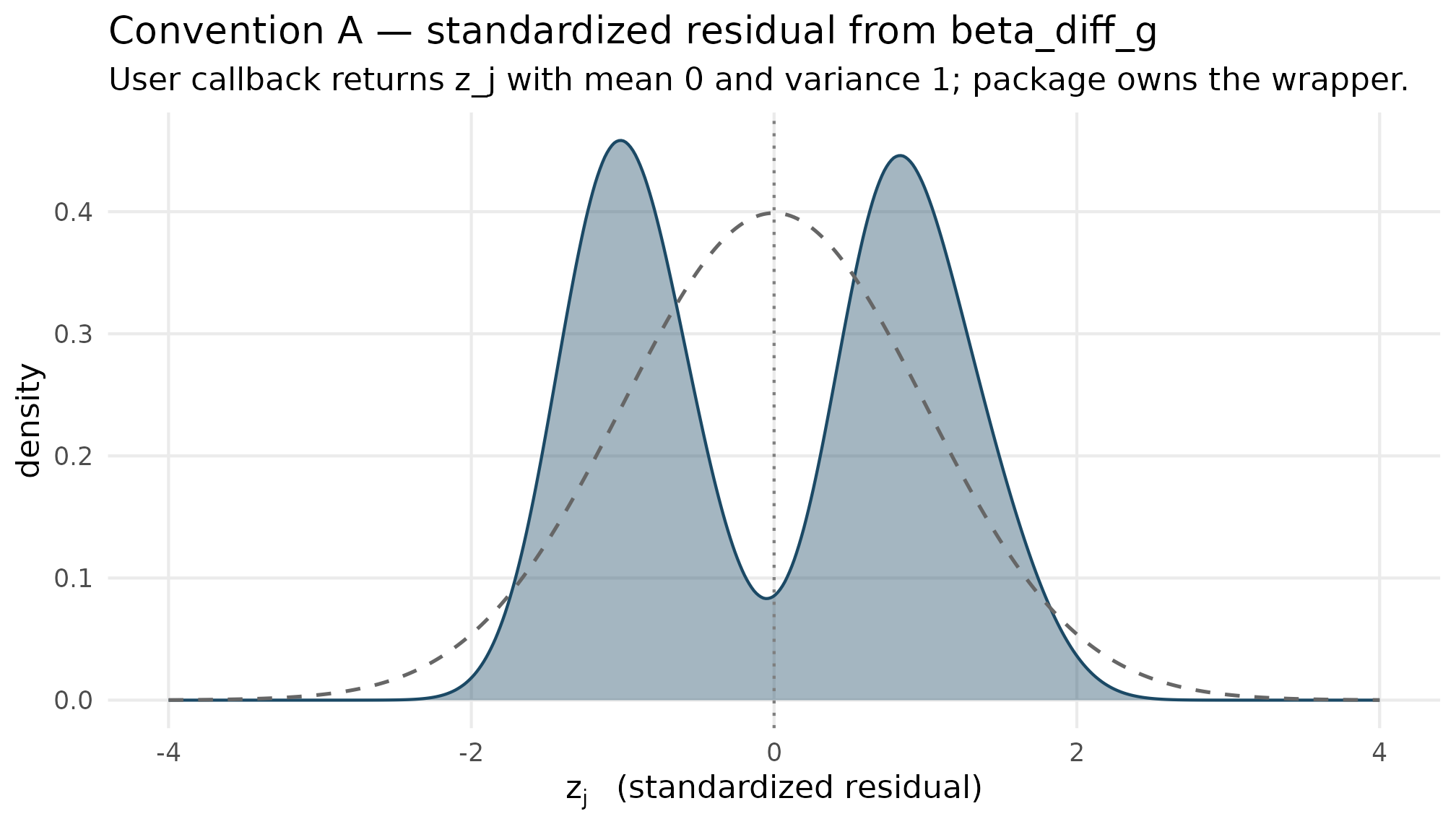

Convention A residual density (blue) over a Gaussian reference (grey dashed). The custom shape is bimodal — the two beta components produce peaks near z = -1 and z = +1 — with thinner tails than Gaussian. Key read: the residual is unit-variance by construction, so the package’s wrapper applied tau + sigma_tau * z_j to produce tau_j the same way it does for any catalog shape.

df_b <- tibble::tibble(tau_j = eff_b$tau_j)
ggplot(df_b, aes(x = tau_j)) +
  geom_histogram(bins = 35, fill = "#62929E",
                 colour = "white", alpha = 0.85) +
  geom_vline(xintercept = 0,    linetype = "dashed", colour = "grey20") +
  geom_vline(xintercept = 0.30, linetype = "dashed", colour = "#1B4965") +
  labs(
    x        = expression(tau[j]~"  (response-scale effect)"),
    y        = "count",
    title    = "Convention B — raw response-scale draw from sparse_g",
    subtitle = "User callback returns tau_j directly; spike at zero, slab around tau = 0.30."
  ) +
  theme_minimal(base_size = 11) +
  theme(panel.grid.minor = element_blank())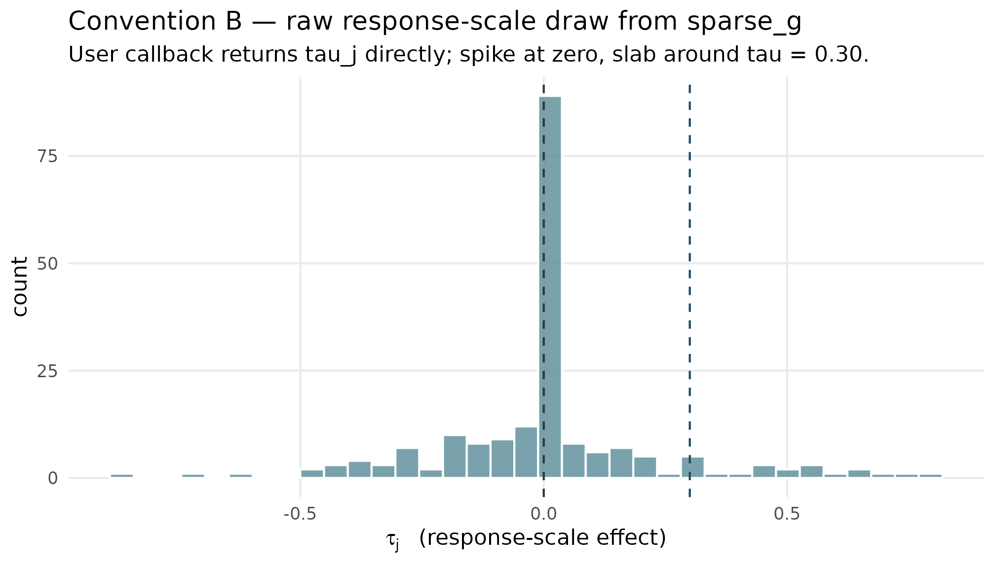

Convention B response-scale tau_j histogram from sparse_g. The exact-zero spike captures about 40 percent of sites (the pi0 weight); the slab portion is Gaussian with SD 0.30 around zero. Dashed lines mark tau and zero. Key read: the callback owns the marginal — the wrapper is bypassed, the spike sits exactly at zero rather than at tau, and the cross-site SD is whatever the slab plus spike produce, not the design’s sigma_tau.

The two plots carry the convention contrast. Convention A lives on the standardized-residual axis, where every shape — catalog or callback — is comparable by construction. Convention B lives on the response scale, where the spike at zero is the substantive feature and the marginal is owned by the callback.

7. Where to next

If, while writing your callback, the shape starts looking like a catalog entry, prefer the catalog. The eight built-in shapes have closed-form unit-variance derivations (where possible) and are exercised at $J = 10^6$ in the test suite — realized variance lands within $10^{-3}$ of 1. A custom callback only matches that guarantee if the standardization step does, and the catalog’s closed-form path is one less moving part to audit. Substantive triggers for the catalog side:

• Symmetric heavy tails — Student-$t$ (gen_effects_studentt()); the closed-form rescaler is exact.
• One-sided skew — skew-normal (gen_effects_skewn()) with the Azzalini slant (Azzalini, 1985).
• Skew with a sharper peak — asymmetric Laplace (gen_effects_ald()) with the Yu-Zhang quantile $\rho$(Yu & Zhang, 2005).
• Two latent classes — two-component mixture (gen_effects_mixture()).
• A fraction of sites exactly null — point-mass-plus-slab (gen_effects_pmslab()), whose $1 / (1 - \pi_0)$ rescaling keeps the residual unit-variance and the diagnostic block clean.

The user-callback path is the right tool when none of these match. Three motifs commonly trigger it: horseshoe-style residuals (sharp peak with very heavy tails — neither Student-$t$ nor ALD captures both), finite mixtures with three or more components, and empirical distributions extracted from a sister study by deconvolution or DPM posterior draws (Lee et al., 2025; Walters, 2024). For the first two, Convention A is the path; for the third, the DPM bridge from Section 5. Sibling vignettes for deeper context: M1: The two-stage DGP (formal specification of the four generative layers — the callback operates inside Layer 1), M2: G-distribution catalog and standardization (the eight built-in shapes and the unit-variance discipline the callback inherits), A8: Cookbook (short walkthroughs that mix custom callbacks with the rest of the design surface), and A5: Calibrating to real data (when calibration against an observed precision distribution suggests a shape outside the catalog).

References

The factorization $\tau_j = \tau + \sigma_\tau z_j$ with a unit-variance standardized residual and the empirical-Bayes context for site-effect estimation are from Lee et al. (2025) and Walters (2024). The catalog parameterizations cross-referenced in the closing pointer are Azzalini (1985) for the skew-normal slant and Yu & Zhang (2005) for the asymmetric Laplace quantile.

Acknowledgments

This research was supported by the Institute of Education Sciences, U.S. Department of Education, through Grant R305D240078 to the University of Alabama. The opinions expressed are those of the authors and do not represent views of the Institute or the U.S. Department of Education.

Session info

#> R version 4.6.0 (2026-04-24)
#> Platform: x86_64-pc-linux-gnu
#> Running under: Ubuntu 24.04.4 LTS
#> 
#> Matrix products: default
#> BLAS:   /usr/lib/x86_64-linux-gnu/openblas-pthread/libblas.so.3 
#> LAPACK: /usr/lib/x86_64-linux-gnu/openblas-pthread/libopenblasp-r0.3.26.so;  LAPACK version 3.12.0
#> 
#> locale:
#>  [1] LC_CTYPE=C.UTF-8       LC_NUMERIC=C           LC_TIME=C.UTF-8       
#>  [4] LC_COLLATE=C.UTF-8     LC_MONETARY=C.UTF-8    LC_MESSAGES=C.UTF-8   
#>  [7] LC_PAPER=C.UTF-8       LC_NAME=C              LC_ADDRESS=C          
#> [10] LC_TELEPHONE=C         LC_MEASUREMENT=C.UTF-8 LC_IDENTIFICATION=C   
#> 
#> time zone: UTC
#> tzcode source: system (glibc)
#> 
#> attached base packages:
#> [1] stats     graphics  grDevices utils     datasets  methods   base     
#> 
#> other attached packages:
#> [1] ggplot2_4.0.3      multisiteDGP_0.1.1
#> 
#> loaded via a namespace (and not attached):
#>  [1] gtable_0.3.6       jsonlite_2.0.0     dplyr_1.2.1        compiler_4.6.0    
#>  [5] tidyselect_1.2.1   nleqslv_3.3.7      jquerylib_0.1.4    systemfonts_1.3.2 
#>  [9] scales_1.4.0       textshaping_1.0.5  yaml_2.3.12        fastmap_1.2.0     
#> [13] R6_2.6.1           labeling_0.4.3     generics_0.1.4     knitr_1.51        
#> [17] tibble_3.3.1       desc_1.4.3         bslib_0.10.0       pillar_1.11.1     
#> [21] RColorBrewer_1.1-3 rlang_1.2.0        cachem_1.1.0       xfun_0.57         
#> [25] fs_2.1.0           sass_0.4.10        S7_0.2.2           cli_3.6.6         
#> [29] pkgdown_2.2.0      withr_3.0.2        magrittr_2.0.5     digest_0.6.39     
#> [33] grid_4.6.0         lifecycle_1.0.5    vctrs_0.7.3        evaluate_1.0.5    
#> [37] glue_1.8.1         farver_2.1.2       ragg_1.5.2         rmarkdown_2.31    
#> [41] tools_4.6.0        pkgconfig_2.0.3    htmltools_0.5.9

Azzalini, A. (1985). A class of distributions which includes the normal ones. Scandinavian Journal of Statistics, 12(2), 171–178.

Lee, J., Che, J., Rabe-Hesketh, S., Feller, A., & Miratrix, L. (2025). Improving the estimation of site-specific effects and their distribution in multisite trials. Journal of Educational and Behavioral Statistics, 50(5), 731–764. https://doi.org/10.3102/10769986241254286

Walters, C. (2024). Empirical bayes methods in labor economics. In Handbook of labor economics (Vol. 5, pp. 183–260). Elsevier. https://doi.org/10.1016/bs.heslab.2024.11.001

Yu, K., & Zhang, J. (2005). A three-parameter asymmetric laplace distribution and its extension. Communications in Statistics — Theory and Methods, 34(9-10), 1867–1879. https://doi.org/10.1080/03610920500199018