Three plot helpers for visualizing a multisitedgp_data simulation.
Each returns a bare ggplot2::ggplot object so the caller can add
themes, labels, facets, or other layers downstream.
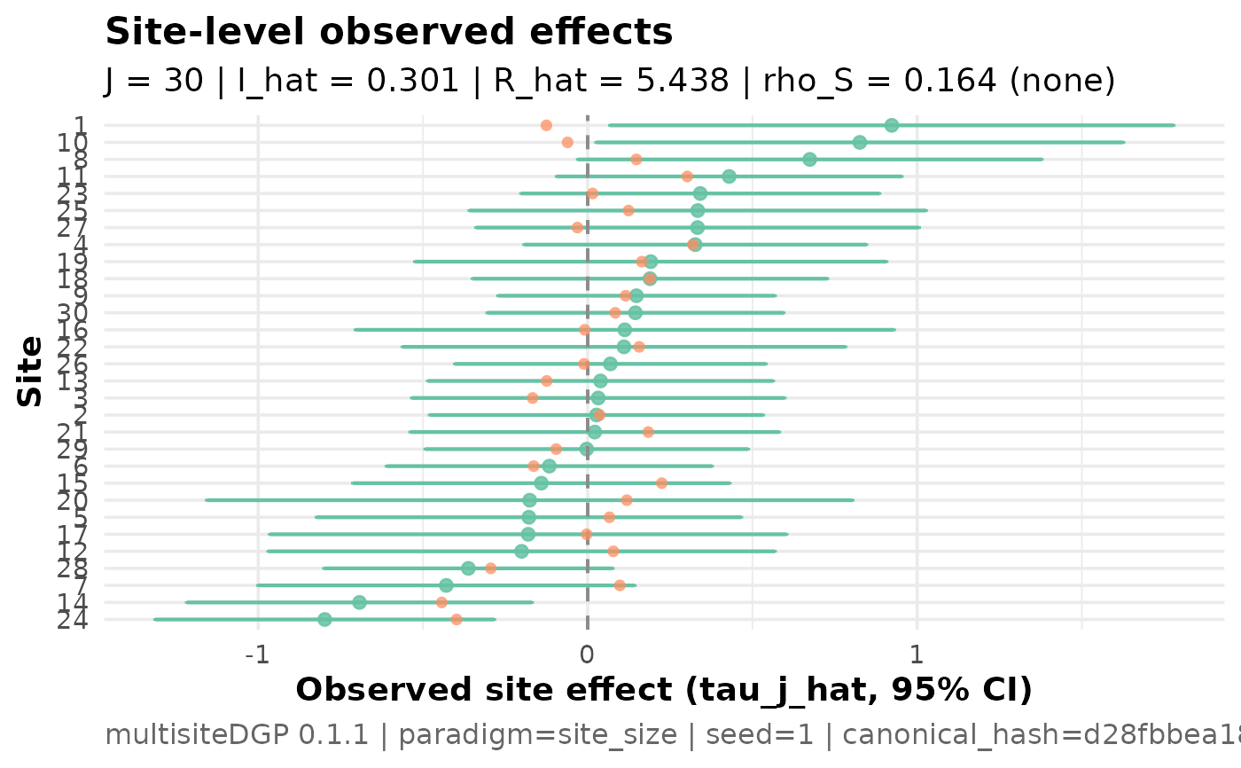
plot_effectsCaterpillar (default) or density view of latent and observed site effects. Use to read off the effect-size ordering and the spread of
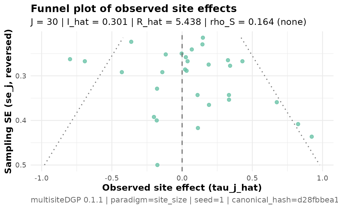
tau_j_hatvstau_j.plot_funnelMeta-analysis funnel —
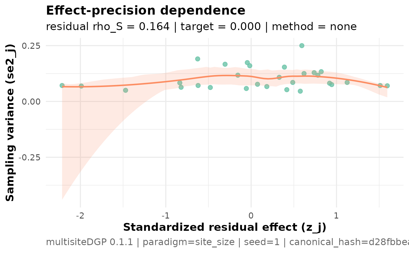
tau_j_hat(x-axis) vsse_j(y-axis, inverted). Use to spot precision-effect dependence and check whether large-SE sites have the same effect distribution as small-SE sites.plot_dependenceScatter of
z_j(ortau_j) againstse2_j. Use to verify that Layer 3 dependence alignment hit its target — the realized rank correlation should match the design.
For the four-question diagnostic rubric and worked applications of these plots, see the A3 Diagnostics in practice vignette. For end-to-end case studies that use these plots, see the A6 multisite trial and A7 meta-analysis case studies.
Usage
plot_effects(
  x,
  type = c("caterpillar", "density"),
  truth = TRUE,
  monochrome = FALSE,
  caption = TRUE,
  ...
)

plot_funnel(
  x,
  reference = c("zero", "tau"),
  envelope = TRUE,
  monochrome = FALSE,
  caption = TRUE,
  ...
)

plot_dependence(
  x,
  smoother = TRUE,
  envelope = TRUE,
  by_residual = TRUE,
  monochrome = FALSE,
  caption = TRUE,
  ...
)
Arguments
- x
A
multisitedgp_dataobject fromsim_multisiteorsim_meta.- type
Character. Effect-plot view —
"caterpillar"(default) or"density".- truth
Logical. Show latent
tau_joverlay alongside observedtau_j_hat. DefaultTRUE.- monochrome
Logical. Use grayscale-safe styling. Default
FALSE.- caption
Logical. Include diagnostic / provenance labels in the plot caption. Default
TRUE.- ...
Reserved for future extensions.
- reference
Character. Funnel reference line —
"zero"(default) or"tau"(the design grand mean).- envelope
Logical. Show the 1.96-SE funnel envelope (the band where 95 percent of estimates would fall under no heterogeneity). Default
TRUE.- smoother
Logical. Add a loess smooth to highlight the trend. Default
TRUE.- by_residual
Logical.
TRUE(default) plots residual-scalez_j;FALSEplots response-scaletau_j. Residual-scale matches the design target of Layer 3 aligners.
Value
A ggplot2::ggplot object.
Functions
plot_effects(): Caterpillar (default) or density view oftau_j_hat(and optionally latenttau_j). Use to read off effect-size ordering and spread.plot_funnel(): Meta-analysis funnel —tau_j_hat(x-axis) vsse_j(y-axis, inverted). Use to spot precision-effect dependence and read whether large-SE sites have the same effect distribution as small-SE sites.plot_dependence(): Scatter of latent effect (z_jby default, ortau_jifby_residual = FALSE) againstse2_j. Use to verify that Layer 3 dependence alignment hit its target — the realized rank correlation should match the design'srank_corr(within Monte Carlo noise).
References
Lee, J., Che, J., Rabe-Hesketh, S., Feller, A., & Miratrix, L. (2025). Improving the estimation of site-specific effects and their distribution in multisite trials. Journal of Educational and Behavioral Statistics, 50(5), 731–764. doi:10.3102/10769986241254286 .
See also
realized_rank_corr, informativeness,
heterogeneity_ratio for scalar diagnostics that
complement the visualizations;
the A3 Diagnostics
in practice vignette.
Examples
dat <- sim_multisite(J = 30L, seed = 1L)
plot_effects(dat)         # caterpillar

plot_funnel(dat)          # funnel

plot_dependence(dat)      # z_j vs se2_j scatter