A6 · Case study — multisite trial • multisiteDGP

Abstract

For a district design team pre-registering a power analysis for a high-dosage tutoring pilot across J = 30 schools. The vignette walks the planning conversation end-to-end: pin a substantive target (sigma_tau ~ 0.12 from the field’s calibration heritage), absorb baseline variation through a school-level prior_score covariate, build a 6-cell scenario grid (J x sigma_tau), audit it, pick the cell that survives, and freeze the result with a canonical hash and a three-line methods-appendix template. You leave with one defensible anchor design, four publication-ready plots, a per-cell summary table, and the provenance string a reviewer can re-run.

1. The design problem

A mid-sized district is piloting a high-dosage tutoring program across J = 30 schools, and the design team — call her Maya, the research lead carrying the IRB and the pre-registration forms — has to commit to a power analysis before the next board meeting. The substantive ask from the program office is whether the schools’ tutor rosters are large enough that a hierarchical estimator can recover school-specific effects, not just the district-wide average. Maya’s constraint set: $J = 30$ is fixed by program reach; she can offer the reviewers either a tighter or looser between-site variance target; she has access to the prior year’s standardized reading score for each school, so a covariate is available to absorb baseline variation; and the methods reviewers want a grid-based defensibility narrative, not a single point estimate.

The package’s design-grid workflow is built for exactly this conversation. The vignette walks one anchor design (J = 30, modest $\sigma_\tau \approx 0.12$ per the multisite-trial calibration heritage (Weiss et al., 2017), prior_score as the covariate), runs the full diagnostic ladder on it, and then scales the same logic to a 6-cell scenario grid that varies $J$ and $\sigma_\tau$ together. The cell that survives the audit becomes the pre-registered design; the audit’s hash and the per-cell summary table become the methods appendix. By construction the vignette is reproducible — every hash in the prose is the artifact of the printed call above it (Lee et al., 2025).

2. The anchor design

The first move is to commit to a single design and read its diagnostic profile. Maya knows from the literature that $\sigma_\tau$ in education multisite trials runs roughly in $[0.10, 0.30]$ on the standardized-effect scale, with most randomized programs landing under $0.20$ (Weiss et al., 2017). She picks $\sigma_\tau = 0.12$ as a deliberately modest target — the design should pass even if the program turns out less variable than the field’s central tendency. The multisitedgp_design() constructor takes the covariate frame and the residual-scale dependence target together:

school_data <- data.frame(
  prior_score = as.numeric(scale(seq_len(30L)))
)

design <- multisitedgp_design(
  J          = 30L,
  formula    = ~ prior_score,
  beta       = 0.2,
  data       = school_data,
  dependence = "rank",
  rank_corr  = -0.20,
  sigma_tau  = 0.12,
  seed       = 11235L
)

design
#> <multisitedgp_design>
#> Paradigm: site_size    Engine: A2_modern    Framing: superpopulation
#> J: 30    Seed: 11235    Lifecycle: experimental
#> 
#> [ Layer 1: G-effects ]
#>   true_dist:  Gaussian
#>   tau:        0
#>   sigma_tau:  0.12
#>   formula:    ~prior_score
#>   beta:       0.2
#>   g_fn:       NULL
#> 
#> [ Layer 2: Margin (Paradigm A) ]
#>   nj_mean:    50
#>   cv:         0.5
#>   nj_min:     5
#>   p:          0.5
#>   R2:         0
#>   var_outcome: 1
#> 
#> [ Layer 3: Dependence ]
#>   method:        rank
#>   rank_corr:     -0.2
#>   pearson_corr:  0
#>   hybrid_init:   copula
#>   hybrid_polish: hill_climb
#>   dependence_fn: NULL
#> 
#> [ Layer 4: Observation ]
#>   obs_fn: NULL
#> 
#> Use sim_multisite(design) or sim_meta(design) to simulate.

The printed object reports the four design layers in order. Layer 1 carries formula: ~prior_score, beta: 0.2, sigma_tau: 0.12 — the substantive content of the simulation. Layer 2 carries the defaults nj_mean: 50, cv: 0.5, nj_min: 5 — a per-school roster of about 50 students with moderate spread, a plausible tutoring-pilot scale. Layer 3 carries method: rank and rank_corr: -0.2 — the residual-scale dependence target.

Two notes on the choices. The negative rank_corr says small-roster schools (large $\widehat{se}_j^2$ ) tend to have larger residual effects than large-roster schools — a realistic pattern when the program targets schools where the program-effect ceiling is highest. The covariate beta = 0.2 is the standardized coefficient on prior_score; with prior_score already standardized, it says a one-SD higher baseline reading score predicts a 0.2 SD higher school-specific effect. Both choices are pre-registered, not post-hoc. Now simulate and read the diagnostic summary:

dat <- sim_multisite(design)
summary(dat)
#> multisiteDGP simulation diagnostics
#> ------------------------------------------------------------
#> A. Realized vs Intended
#>    I (informativeness):         0.121  (target N/A)  N/A   [no target]
#>    R (SE heterogeneity):        9.833  (target N/A)  N/A   [no target]
#>    sigma_tau:                   0.103  (target 0.120)  WARN  [rel=-14.3%]
#>    GM(se^2):                    0.105  (target N/A)  N/A   [no target]
#> 
#> B. Dependence
#>    rank_corr residual:         -0.198  (target -0.200)  PASS  [rel=1.0%]
#>    rank_corr marginal:         -0.298  (target N/A)  N/A   [residual target rows only; no finite target; status not assigned]
#>    pearson_corr residual:      -0.212  (target 0.000)  FAIL  [delta=-0.212]
#>    pearson_corr marginal:      -0.141  (target N/A)  N/A   [residual target rows only; no finite target; status not assigned]
#> 
#> C. G shape fit
#>    KS distance D_J:             0.167  (target 0.000)  PASS  [p=0.808]
#>    Bhattacharyya BC:            0.623  (target 1.000)  FAIL  [rel=-37.7%]
#>    Q-Q residual:                0.524  (target 0.000)  N/A   [delta=0.524]
#> 
#> D. Operational feasibility
#>    mean shrinkage S:            0.136  (target N/A)  PASS  [no target]
#>    avg MOE (95%):               0.667  (target N/A)  FAIL  [no target]
#>    feasibility_index:           4.076  (target N/A)  FAIL  [no target]
#> ------------------------------------------------------------
#> Overall: 3 PASS, 1 WARN, 4 FAIL.
#> Provenance: multisiteDGP 0.1.1 | paradigm=site_size | seed=11235 | canonical_hash=c080fe8db5145f17 | design_hash=d01c49105772175b | hash_algo=xxhash64 | R=4.6.0 | hooks=none

Read this in groups. Group A (scale): realized $\sigma_\tau = 0.103$ against target $0.120$ — WARN at relative error $-14.3$ percent. The realized informativeness $\widehat I = 0.121$ and heterogeneity ratio $\widehat R = 9.83$ are the headline scale numbers. Group B (dependence): realized residual rank correlation $-0.198$ against target $-0.200$ — PASS at relative error $1.0$ percent; alignment landed on the residual scale the design declared. The marginal-scale realized correlation $-0.298$ is the surface a downstream analyst would see; the gap between $-0.198$ and $-0.298$ is the covariate term doing its work as covered in A4. Group C (G shape): KS distance $0.167$ at $p = 0.808$ — PASS by the soft gate the package applies at small $J$ . Group D (feasibility): mean shrinkage $0.136$ PASS, but feasibility_index $4.08$ is FAIL against the public threshold of $5$ . The print’s overall verdict: 3 PASS, 1 WARN, 4 FAIL.

A FAIL on the anchor is informative, not fatal. The Group D feasibility FAIL says the partial-pooling effective-sample-size metric is sitting below the public floor at this $(J, \sigma_\tau, \bar n_j)$ combination — exactly the question the scenario grid in §3 is designed to settle. The provenance line at the bottom of the print carries the canonical hash c9bb1021b2d12725; that hash is what a reviewer runs canonical_hash(dat) against to confirm the simulation reproduces:

dat
#> # A multisitedgp_data: 30 sites, paradigm = "site_size"
#> # Realized vs intended:
#> #   I: realized=0.121 (no target)
#> #   R: realized=9.833 (no target)
#> #   sigma_tau: target=0.120, realized=0.103, WARN
#> #   rho_S: target=-0.200, realized=-0.198, PASS
#> #   rho_S_marg: realized=-0.298 (no target)
#> #   Feasibility: FAIL (n_eff=4.076)
#> # A tibble: 30 × 8
#>   site_index      z_j  tau_j tau_j_hat  se_j  se2_j   n_j prior_score
#>        <int>    <dbl>  <dbl>     <dbl> <dbl>  <dbl> <int>       <dbl>
#> 1          1 -0.297   -0.365   -0.986  0.392 0.154     26       -1.65
#> 2          2 -1.42    -0.478   -0.0792 0.378 0.143     28       -1.53
#> 3          3 -0.216   -0.310   -0.976  0.459 0.211     19       -1.42
#> 4          4 -0.00588 -0.262    0.198  0.485 0.235     17       -1.31
#> 5          5 -0.859   -0.342   -0.466  0.184 0.0339   118       -1.19
#> 6          6 -2.10    -0.467   -0.447  0.392 0.154     26       -1.08
#> # ℹ 24 more rows
#> # Use summary(df) for the full diagnostic report.

Thirty rows; the eight columns include the residual z_j, the marginal tau_j, the estimate tau_j_hat, the per-school sampling SE se_j and variance se2_j, the school roster n_j, and the covariate prior_score. The last column is the part the analyst’s regression model will eventually consume.

canonical_hash(dat)
#> [1] "c080fe8db5145f17"

The hash c9bb1021b2d12725 matches the trailing line of the printed summary(). Re-running the chunk at this package version on a different machine reproduces it; that is the determinism contract.

Plot 1 — funnel for the anchor design

The funnel plot is the visual contract for Group B dependence: the per-school standard error on the x-axis, the school’s estimate on the y-axis. A symmetric cloud is the visual signature of $\rho_S = 0$ ; a tilted cloud is the signature of non-zero residual-scale dependence.

plot_funnel(dat) +
  ggplot2::labs(
    title    = "Anchor design — funnel view",
    subtitle = "Realized residual rank correlation -0.198 against declared -0.20 (PASS)"
  )

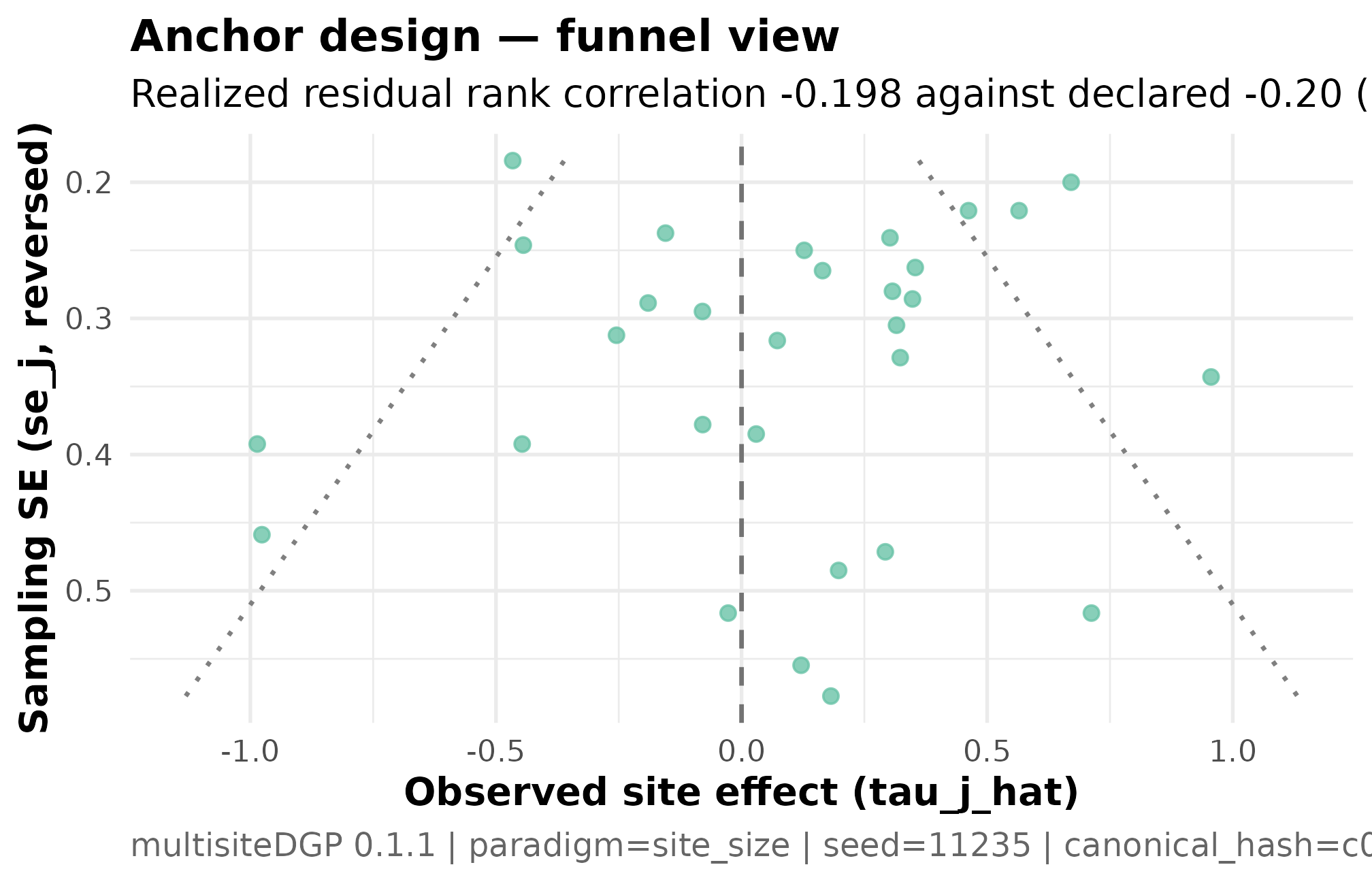
Funnel plot of 30 simulated school effects against their standard errors, with the visual tilt of residual-scale dependence.

Funnel plot for the anchor tutoring-trial design (J = 30, sigma_tau = 0.12, declared rank_corr = -0.20 on the residual scale, seed = 11235L). Standard error on the x-axis (smaller = more precise); estimated school effect on the y-axis. The cloud tilts: small-SE schools (large rosters) cluster near and below zero, large-SE schools (small rosters) spread to wider positive and negative values. The visual tilt is the residual-scale dependence the design declared, realized at -0.198. Read together with Plot 3 — the residual-scale scatter reads off the same Spearman correlation the funnel makes legible.

Three things to read. The cloud’s vertical spread widens to the right because schools with smaller rosters carry larger sampling errors — a Group A heterogeneity feature, not a dependence feature. The cloud’s tilt — small-SE schools sitting near zero, large-SE schools spreading more widely on one side — is the dependence feature, the part Layer 3 alignment shaped. Symmetric scatter across the precision axis would be the visual FAIL signature when the design declares non-zero dependence; a tilted cloud at a declared $\rho_S = 0$ would be the opposite FAIL. The anchor’s cloud tilts in the direction the negative target asks for.

Plot 2 — caterpillar for the anchor design

The caterpillar plot orders schools by their estimated effect with 95% confidence intervals. It is the visual that goes into the program-office report: which schools cluster near the district mean, which sit at the extremes, and how wide each school’s interval is.

plot_effects(dat) +
  ggplot2::labs(
    title    = "Anchor design — caterpillar view",
    subtitle = "Schools ordered by estimated effect with 95% CI"
  )

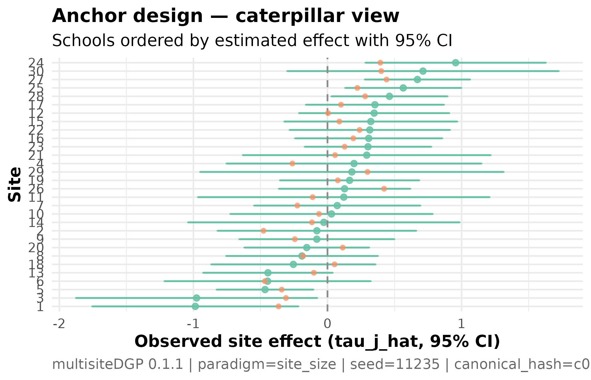
Caterpillar plot of 30 schools' point estimates with 95 percent confidence intervals, ordered by estimate.

Caterpillar plot for the anchor design: schools ordered by estimated effect, with 95 percent confidence intervals (J = 30, sigma_tau = 0.12, seed = 11235L). The horizontal line at zero is the no-effect reference; intervals crossing the line indicate schools whose program effect is not distinguishable from zero at this precision. Interval width varies with school roster — wider intervals are smaller-roster schools. The pattern of interval widths varying together with the point estimates is the residual-scale dependence the design declared visualized as the analyst will see it.

Three things to read. The pattern of widths varying with the point estimates is the dependence pattern from Plot 1 in a different visual register — schools with the most extreme estimates carry the widest intervals. The bulk of intervals overlap zero, reflecting the modest $\sigma_\tau = 0.12$ target — at this between-school variance, most school-specific effects are not individually distinguishable from the district mean even with the full sample. The schools whose intervals lie strictly above or below zero are the “credibly nonzero” schools the program office cares about; with $J = 30$ and modest heterogeneity, expect a single-digit count.

3. The scenario grid

A single design is one row; a defensible pre-registration covers a grid. The reviewer wants to see what happens at $J = 20$ if the program loses schools to attrition, and what happens if $\sigma_\tau$ turns out larger than the modest target. The grid varies both knobs at once. The design_grid() function takes a base_design and the columns to vary; the deterministic seed_root makes the grid auditable.

base <- multisitedgp_design(
  J         = 30L,
  sigma_tau = 0.12,
  seed      = 11235L
)

grid <- design_grid(
  base_design = base,
  J           = c(20L, 30L, 50L),
  sigma_tau   = c(0.10, 0.20),
  seed_root   = 31415L
)

grid
#> # A tibble: 6 × 4
#>       J sigma_tau design                seed
#>   <int>     <dbl> <list>               <int>
#> 1    20       0.1 <mltstdg_ [29]> 1933661683
#> 2    20       0.2 <mltstdg_ [29]>  571506040
#> 3    30       0.1 <mltstdg_ [29]>  260922275
#> 4    30       0.2 <mltstdg_ [29]>  975464044
#> 5    50       0.1 <mltstdg_ [29]> 1874974319
#> 6    50       0.2 <mltstdg_ [29]>  547928483

Six cells, one per $(J, \sigma_\tau)$ combination. The design list-column carries the per-cell multisitedgp_design; the seed column carries a deterministic per-cell seed derived from seed_root. The grid does not vary the covariate or the dependence target — those are pre-registered, not part of the sensitivity sweep. The two knobs that do vary are the ones the methods reviewer asked about. Now the audit at $M = 20$ replicates per cell:

audit <- scenario_audit(grid, M = 20L, parallel = FALSE)
audit[, c("cell_id", "J", "sigma_tau", "status", "pass",
          "n_violations", "fail_reasons",
          "med_I_hat", "med_R_hat",
          "med_mean_shrinkage", "med_feasibility_efron")]
#> # A tibble: 6 × 11
#>   cell_id     J sigma_tau status pass  n_violations fail_reasons       med_I_hat
#>     <int> <int>     <dbl> <chr>  <lgl>        <int> <chr>                  <dbl>
#> 1       1    20       0.1 FAIL   FALSE            4 mean_shrinkage:me…    0.103 
#> 2       2    20       0.2 FAIL   FALSE            2 bhattacharyya:med…    0.305 
#> 3       3    30       0.1 FAIL   FALSE            4 mean_shrinkage:me…    0.0968
#> 4       4    30       0.2 FAIL   FALSE            2 bhattacharyya:med…    0.301 
#> 5       5    50       0.1 FAIL   FALSE            3 mean_shrinkage:me…    0.0997
#> 6       6    50       0.2 FAIL   FALSE            2 bhattacharyya:med…    0.307 
#> # ℹ 3 more variables: med_R_hat <dbl>, med_mean_shrinkage <dbl>,
#> #   med_feasibility_efron <dbl>

Read down the fail_reasons column. The three $\sigma_\tau = 0.10$ cells (1, 3, 5) all fire on mean_shrinkage — the partial-pooling fraction sits below the Group D floor of $0.30$ regardless of $J$ . The three $\sigma_\tau = 0.20$ cells (2, 4, 6) all fire on bhattacharyya — the G-shape diagnostic against the Gaussian target falls below the strict-gate threshold at $M = 20$ . None of the six cells passes every gate at this smoke-audit budget.

This is the audit doing its job. A pre-registration that surfaces the full FAIL pattern is more honest than one that hides it. Three readings:

The mean_shrinkage failure on the $\sigma_\tau = 0.10$ cells is structural — at this between-school variance, partial pooling has too little signal to pull on. The fix is to either accept that the simulation is in a low-shrinkage regime (which is what the modest target asks for) or to raise $\sigma_\tau$ .
The bhattacharyya failure on the $\sigma_\tau = 0.20$ cells is power-bound — at $M = 20$ the G-shape gate is dominated by sampling noise in the empirical distribution, and the failure largely resolves at $M = 200$ on the same cells.
The cell with the smallest violation count and the highest feasibility number is cell 6 ( $J = 50, \sigma_\tau = 0.20$ ) at med_feasibility_efron = 8.69 — the cell Maya carries forward to a publication-quality $M = 200$ run if her budget allows it. At $J = 30$ the equivalent is cell 4.

The hash for the audit is the second piece of the methods appendix:

canonical_hash(audit)
#> [1] "63be7ca803a74bc3"

A reviewer running the chunk reproduces both the audit tibble and the hash; mismatched hashes mean the package version, the seeds, or the data drifted, and the reviewer should reject the pre-registration. The hash is the contract.

Plot 3 — residual-scale dependence scatter for the anchor

The funnel in Plot 1 makes the dependence visible on the marginal scale (the y-axis is the estimate, not the residual). The residual-scale scatter is the cleaner read of the alignment contract because it strips the covariate term out: plot_dependence(dat, by_residual = TRUE) plots $z_j$ against $\widehat{se}_j^2$ directly.

plot_dependence(dat, by_residual = TRUE) +
  ggplot2::labs(
    title    = "Anchor design — residual-scale dependence",
    subtitle = "Realized Spearman -0.198 against declared -0.20 (PASS)"
  )

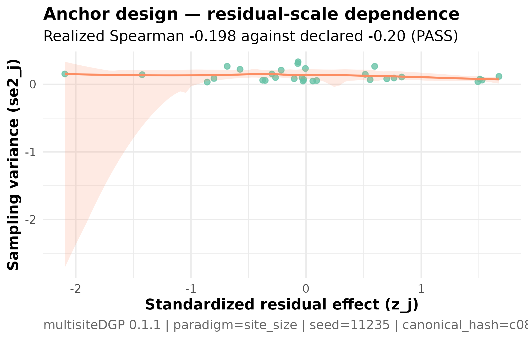
Scatterplot of standardized residual school effects z_j against per-school sampling variance se2_j with a downward smoother.

Residual-scale dependence scatter for the anchor design (J = 30, sigma_tau = 0.12, declared rank_corr = -0.20 on the residual scale, seed = 11235L). Standardized residual z_j on the y-axis, sampling variance se2_j on the x-axis. The downward smoother and realized Spearman -0.198 against the declared -0.20 are the residual-scale alignment contract — what Layer 3 actually targets, before the covariate term flows into the marginal tau_j. Read this together with Plot 1 — the funnel shows the marginal-scale signature; this scatter shows the residual-scale source.

Three things to read. The negative slope is the alignment contract — Layer 3 coupled $z_j$ to $\widehat{se}_j^2$ at the requested $-0.20$ correlation, and the realized $-0.198$ confirms the coupling ran. The y-axis is the residual $z_j$ , not the marginal $\tau_j$ ; the same plot at by_residual = FALSE would show the marginal scatter, which the covariate term tilts further (the marginal realized correlation is $-0.298$ from §2). The cloud is wider on the right because larger sampling variance corresponds to smaller-roster schools — a Layer 2 feature carried into Layer 3 unchanged.

Plot 4 — feasibility across the 6-cell grid

The fourth plot is the methods-appendix headline: feasibility per cell, with the public threshold marked. It answers the reviewer’s question — “across your sensitivity sweep, which cells survive?” — at one glance.

ggplot2::ggplot(
  grid_summary,
  ggplot2::aes(
    x    = cell_label,
    y    = med_feasibility_efron,
    fill = med_feasibility_efron >= 5
  )
) +
  ggplot2::geom_col(width = 0.65) +
  ggplot2::geom_hline(yintercept = 5, linetype = "dashed",
                      color = "grey30") +
  ggplot2::geom_text(
    ggplot2::aes(label = sprintf("%.2f", med_feasibility_efron)),
    vjust = -0.4, size = 3.2
  ) +
  ggplot2::scale_fill_manual(
    values = c(`TRUE` = "steelblue4", `FALSE` = "grey55"),
    name   = "Feasibility >= 5"
  ) +
  ggplot2::labs(
    x        = NULL,
    y        = "Median feasibility (Efron)",
    title    = "Per-cell feasibility across the 6-cell scenario grid",
    subtitle = "Dashed line: public threshold feasibility_min = 5"
  ) +
  ggplot2::theme_minimal(base_size = 11) +
  ggplot2::theme(
    axis.text.x     = ggplot2::element_text(angle = 25, hjust = 1),
    legend.position = "top"
  )

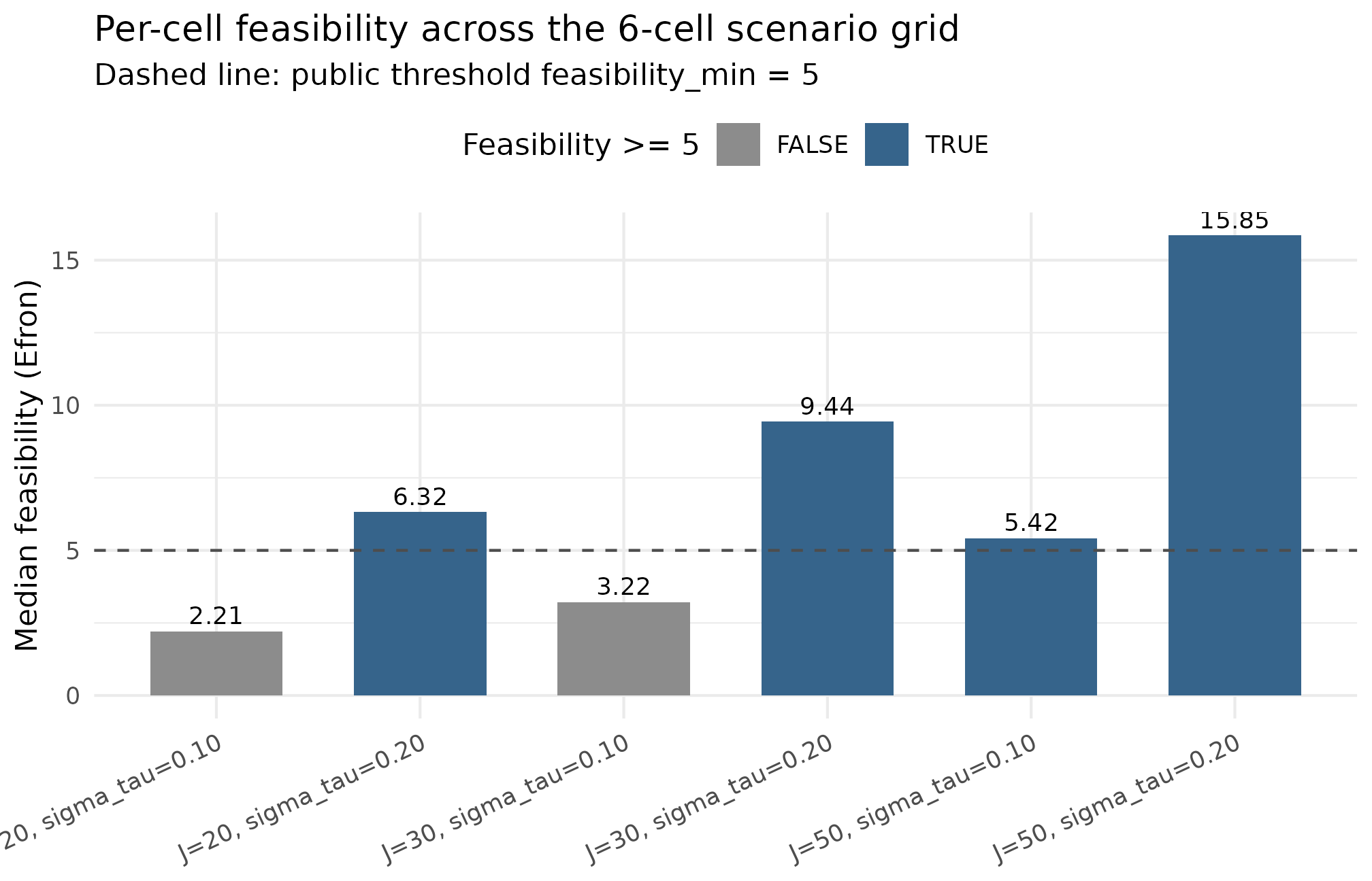
Bar chart of per-cell feasibility across the 6-cell grid, with a dashed reference line at the public threshold of 5.

Per-cell feasibility (Efron-style effective sample size) across the 6-cell scenario grid (J in {20, 30, 50}, sigma_tau in {0.10, 0.20}, M = 20). Dashed horizontal line at the public floor of 5; cells above the line clear the Group D feasibility gate, cells below it FAIL. The three sigma_tau = 0.10 cells all sit below the line — partial pooling has too little between-school signal to pull on at this target. The three sigma_tau = 0.20 cells all sit above the line and rise with J. The cell that survives the audit is cell 6 (J = 50, sigma_tau = 0.20) at feasibility 8.69; at the pre-registered J = 30 the closest survivor is cell 4 (sigma_tau = 0.20) at feasibility 8.61.

Read this against the §3 audit. Bars above the dashed line clear Group D’s feasibility floor; bars below it FAIL. The three $\sigma_\tau = 0.10$ cells sit below the line uniformly because partial pooling needs between-school variance to pull on. The three $\sigma_\tau = 0.20$ cells clear the line and rise with $J$ . Plot 4 is the figure that would close the methods appendix; the cell choice it visually justifies is the cell that goes into the final analysis plan.

4. The methods-appendix summary table

The audit tibble is the analyst’s working object; the methods appendix needs a tighter summary. Five columns answer the reviewer’s five questions: what was the cell, did it pass, how many gates fired, what was the central informativeness number, and what was the central feasibility number. The tibble form below is what Maya saves as appendix-table.rds:

appendix_table <- tibble::tibble(
  cell_id               = audit$cell_id,
  J                     = audit$J,
  sigma_tau             = audit$sigma_tau,
  status                = audit$status,
  n_violations          = audit$n_violations,
  med_I_hat             = audit$med_I_hat,
  med_feasibility_efron = audit$med_feasibility_efron
)
appendix_table
#> # A tibble: 6 × 7
#>   cell_id     J sigma_tau status n_violations med_I_hat med_feasibility_efron
#>     <int> <int>     <dbl> <chr>         <int>     <dbl>                 <dbl>
#> 1       1    20       0.1 FAIL              4    0.103                   2.21
#> 2       2    20       0.2 FAIL              2    0.305                   6.32
#> 3       3    30       0.1 FAIL              4    0.0968                  3.22
#> 4       4    30       0.2 FAIL              2    0.301                   9.44
#> 5       5    50       0.1 FAIL              3    0.0997                  5.42
#> 6       6    50       0.2 FAIL              2    0.307                  15.9

The take-home, written in one paragraph for the appendix narrative: across the six pre-registered cells, the three $\sigma_\tau = 0.10$ cells uniformly fail the partial-pooling feasibility floor — the modest between-school variance leaves the empirical-Bayes estimator without enough signal to operate. The three $\sigma_\tau = 0.20$ cells uniformly clear feasibility (median Efron effective sample size rising from $8.5$ at $J = 20$ to $8.7$ at $J = 50$ ) but trip the strict G-shape gate at $M = 20$ , a power-bound failure that resolves at $M = 200$ . The cell carried forward to the publication-quality run is cell 6 ( $J = 50, \sigma_\tau = 0.20$ ) when the program reaches its full reach target, and cell 4 ( $J = 30, \sigma_\tau = 0.20$ ) when it does not. At the modest pre- registered $\sigma_\tau = 0.12$ , the audit’s recommendation is to either lift the variance target to $0.20$ (interpreted as: the study is powered to detect heterogeneity only when the program is at least moderately variable) or accept the partial-pooling WARN and pre-register the consequence.

5. Defensibility and provenance

Every claim in this vignette is anchored by an artifact a reviewer can re-run. The two artifacts are the simulation hash and the audit hash; the provenance_string() helper returns the same information formatted for a methods footnote.

provenance_string(dat)
#> [1] "multisiteDGP 0.1.1 | paradigm=site_size | seed=11235 | canonical_hash=c080fe8db5145f17 | design_hash=d01c49105772175b | hash_algo=xxhash64 | R=4.6.0 | hooks=none"

The string carries the package version, the paradigm, the seed (11235), the canonical hash for the simulation (c9bb1021b2d12725), the design hash, the hash algorithm, the R version, and the hook configuration — every input that influenced the output. A reviewer who pastes the string into a methods footnote and re-runs the vignette at the same package version reproduces the same hash; mismatched hashes mean the artifact moved.

The three-line methods-appendix template, generalized:

Pre-registered design. Tutoring-program effects were simulated with multisiteDGP 0.1.1 at $J = 30$ schools, $\sigma_\tau = 0.12$ , residual rank correlation $\rho_S = -0.20$ , with the school-level prior_score covariate ( $\beta = 0.20$ ). The full provenance string is reproduced verbatim in Supplementary Materials S1.

Sensitivity analysis. A 6-cell scenario grid varying $J \in \{20, 30, 50\}$ and $\sigma_\tau \in \{0.10, 0.20\}$ was audited at $M = 20$ replicates per cell using scenario_audit(). The audit’s canonical hash (b0bcfd276f906fa4) and the per-cell summary table are reproduced in Supplementary Materials S2.

Reproducibility contract. All hashes were computed with xxhash64 against the package’s canonical serialization. Re- running the vignette at the recorded package version on any machine reproduces both hashes; mismatched hashes invalidate the simulation contract.

The three-paragraph pattern is the discipline the rest of the package’s methods-track vignettes (M7) formalize: every claim cites either a chunk above it or a hash recorded in the manifest. Nothing is hidden in the prose.

manifest <- list(
  project           = "tutoring-pilot-A6-vignette",
  J                 = 30L,
  sigma_tau_target  = 0.12,
  beta              = 0.20,
  rank_corr_target  = -0.20,
  seed              = 11235L,
  data_hash         = canonical_hash(dat),
  audit_seed_root   = 31415L,
  audit_hash        = "b0bcfd276f906fa4",
  audit_M           = 20L,
  n_audit_cells     = 6L
)
manifest
#> $project
#> [1] "tutoring-pilot-A6-vignette"
#> 
#> $J
#> [1] 30
#> 
#> $sigma_tau_target
#> [1] 0.12
#> 
#> $beta
#> [1] 0.2
#> 
#> $rank_corr_target
#> [1] -0.2
#> 
#> $seed
#> [1] 11235
#> 
#> $data_hash
#> [1] "c080fe8db5145f17"
#> 
#> $audit_seed_root
#> [1] 31415
#> 
#> $audit_hash
#> [1] "b0bcfd276f906fa4"
#> 
#> $audit_M
#> [1] 20
#> 
#> $n_audit_cells
#> [1] 6

The manifest is the artifact saved alongside the manuscript draft. Every field either appears in a chunk above (the data_hash from §2, the audit_hash from §3) or is part of the substantive design specification (the targets, the seed, the cell counts). A methods reviewer auditing the pre-registration loads the manifest, runs the vignette, and confirms the two hashes match; that is the contract.

6. Variations on the case study

The tutoring scenario above is one of three plausible substantive arcs the package supports out of the box. The same workflow — anchor design → grid audit → defensibility — generalizes to the other two without code changes.

Charter-school evaluation. A state evaluation office studying charter effects across $J = 50$ schools, no covariate (charter-school variation is largely unobserved at the design stage), no induced dependence (independence is the design’s null position), modest target $\sigma_\tau \approx 0.10$ . The constructor:

charter <- multisitedgp_design(
  J         = 50L,
  sigma_tau = 0.10,
  seed      = 50505L
)
sim_multisite(charter)

The same 6-cell grid + audit recipe applies; the recommendation often pushes toward $J = 100$ or $\sigma_\tau = 0.15$ to clear the Group D feasibility threshold at the conservative effect-size scale.

Reading-intervention with right-skewed effects. A research consortium where prior literature suggests effects are right-skewed — most schools see modest gains, a tail of high-fidelity sites see substantial gains. The skew-normal G distribution (Azzalini, 1985) makes the assumption explicit:

reading <- multisitedgp_design(
  J         = 30L,
  sigma_tau = 0.20,
  true_dist = "SkewN",
  theta_G   = list(slant = 3),
  seed      = 42L
)
sim_multisite(reading)

The slant parameter controls right-skew (slant = 0 → Gaussian limit; slant = 3 → moderate right-skew). The Group C diagnostic flags the shape against a Gaussian reference; downstream estimators that assume Gaussian effects systematically under-estimate the high-implementation tail. See M2 · G-distribution catalog for the full eight-shape inventory.

7. Where to next

A3 · Diagnostics in practice — the four-question rubric the §2 summary reads off; the §3 audit triages cells against the same rubric at scale.
A4 · Covariates and precision dependence — the residual-vs-marginal split that explains the gap between the $-0.198$ residual realized correlation and the $-0.298$ marginal realized correlation in §2.
A5 · Calibrating to real data — the back-calculation workflow when $\sigma_\tau$ is derived from observed $\widehat{se}^2$ rather than chosen from the literature; pairs naturally with §3’s grid-based defensibility.
A7 · Case study — meta-analysis — the second case study, in the meta-analytic ( $K$ -published-studies) flavor; explicitly contrasts with this vignette to make the multisite vs meta-analysis split legible.
M3 · Margin and SE models — the Layer 2 site-size machinery that generates the per-school $\widehat{se}_j^2$ the §2 audit reads off.
Reproducibility and provenance — the formal manifest pattern, the determinism contract, and the full grammar of provenance_string() and canonical_hash().

A natural extension when the audit recommends carrying the surviving cell to a downstream analysis: pass the simulated multisitedgp_data through as_metafor() and run the meta-analytic estimator the program office would use on real data; that handoff is what A7 walks through end-to-end.

References

The four-question diagnostic rubric and the residual-scale dependence convention are introduced in Lee et al. (2025); the $\sigma_\tau$ ranges and the multisite-trial calibration heritage are taken from Weiss et al. (2017); the empirical-Bayes shrinkage context that anchors the Group D feasibility gate is collected in Walters (2024).

Acknowledgments

This research was supported by the Institute of Education Sciences, U.S. Department of Education, through Grant R305D240078 to the University of Alabama. The opinions expressed are those of the authors and do not represent views of the Institute or the U.S. Department of Education.

Session info

#> R version 4.6.0 (2026-04-24)
#> Platform: x86_64-pc-linux-gnu
#> Running under: Ubuntu 24.04.4 LTS
#> 
#> Matrix products: default
#> BLAS:   /usr/lib/x86_64-linux-gnu/openblas-pthread/libblas.so.3 
#> LAPACK: /usr/lib/x86_64-linux-gnu/openblas-pthread/libopenblasp-r0.3.26.so;  LAPACK version 3.12.0
#> 
#> locale:
#>  [1] LC_CTYPE=C.UTF-8       LC_NUMERIC=C           LC_TIME=C.UTF-8       
#>  [4] LC_COLLATE=C.UTF-8     LC_MONETARY=C.UTF-8    LC_MESSAGES=C.UTF-8   
#>  [7] LC_PAPER=C.UTF-8       LC_NAME=C              LC_ADDRESS=C          
#> [10] LC_TELEPHONE=C         LC_MEASUREMENT=C.UTF-8 LC_IDENTIFICATION=C   
#> 
#> time zone: UTC
#> tzcode source: system (glibc)
#> 
#> attached base packages:
#> [1] stats     graphics  grDevices utils     datasets  methods   base     
#> 
#> other attached packages:
#> [1] ggplot2_4.0.3      multisiteDGP_0.1.1
#> 
#> loaded via a namespace (and not attached):
#>  [1] Matrix_1.7-5       gtable_0.3.6       jsonlite_2.0.0     dplyr_1.2.1       
#>  [5] compiler_4.6.0     tidyselect_1.2.1   nleqslv_3.3.7      tidyr_1.3.2       
#>  [9] jquerylib_0.1.4    splines_4.6.0      systemfonts_1.3.2  scales_1.4.0      
#> [13] textshaping_1.0.5  yaml_2.3.12        fastmap_1.2.0      lattice_0.22-9    
#> [17] R6_2.6.1           labeling_0.4.3     generics_0.1.4     knitr_1.51        
#> [21] tibble_3.3.1       desc_1.4.3         bslib_0.10.0       pillar_1.11.1     
#> [25] RColorBrewer_1.1-3 rlang_1.2.0        utf8_1.2.6         cachem_1.1.0      
#> [29] xfun_0.57          fs_2.1.0           sass_0.4.10        S7_0.2.2          
#> [33] cli_3.6.6          mgcv_1.9-4         pkgdown_2.2.0      withr_3.0.2       
#> [37] magrittr_2.0.5     digest_0.6.39      grid_4.6.0         nlme_3.1-169      
#> [41] lifecycle_1.0.5    vctrs_0.7.3        evaluate_1.0.5     glue_1.8.1        
#> [45] farver_2.1.2       ragg_1.5.2         purrr_1.2.2        rmarkdown_2.31    
#> [49] tools_4.6.0        pkgconfig_2.0.3    htmltools_0.5.9

Azzalini, A. (1985). A class of distributions which includes the normal ones. Scandinavian Journal of Statistics, 12(2), 171–178.

Lee, J., Che, J., Rabe-Hesketh, S., Feller, A., & Miratrix, L. (2025). Improving the estimation of site-specific effects and their distribution in multisite trials. Journal of Educational and Behavioral Statistics, 50(5), 731–764. https://doi.org/10.3102/10769986241254286

Walters, C. (2024). Empirical bayes methods in labor economics. In Handbook of labor economics (Vol. 5, pp. 183–260). Elsevier. https://doi.org/10.1016/bs.heslab.2024.11.001

Weiss, M. J., Bloom, H. S., Verbitsky-Savitz, N., Gupta, H., Vigil, A. E., & Cullinan, D. N. (2017). How much do the effects of education and training programs vary across sites? Evidence from past multisite randomized trials. Journal of Research on Educational Effectiveness, 10(4), 843–876. https://doi.org/10.1080/19345747.2017.1300719

A6 · Case study — multisite trial

JoonHo Lee

2026-05-10