A3 · Diagnostics in practice

JoonHo Lee

2026-05-10

Abstract

For methodologists who can already run sim_multisite() and now need to decide whether the realized design is fit for the analysis that follows. This vignette walks the four-question diagnostic rubric on a single working design — scale, dependence, G-shape, feasibility — showing the function that answers each question, the plot that makes the answer legible, and the design move that fixes it when the answer comes back red. You leave with a one-page triage card mapping each red status to the change it implies, and a scenario_audit() call that scales the same logic across a design grid.

1. The four questions

A multisite simulation is only useful if four things land where the designer asked. The four diagnostic groups answer one question each; every Group A/B/C/D row in summary(dat) is a PASS / WARN / FAIL verdict on one of them (Lee et al., 2025).

Group	Question	Lead helpers	Threshold source
A	Did the simulation reach the target information scale?	informativeness(), heterogeneity_ratio(), compute_I(), compute_kappa()	feasibility_min, R_max
B	Did the precision–effect dependence land where the design asked?	realized_rank_corr(), realized_rank_corr_marginal()	qualitative (compare to design rank_corr)
C	Does the realized G shape match the target distribution?	bhattacharyya_coef(), ks_distance()	bhattacharyya_min, ks_max
D	Will the design work downstream — is shrinkage non-trivial?	mean_shrinkage(), feasibility_index(), default_thresholds()	mean_shrinkage_min, feasibility_min

The rest of this vignette is a reference card: one section per group with the call signatures, the ground-truth values for preset_jebs_paper(seed = 1L), what to read off the diagnostic plot, and the design move that fixes it when the answer comes back red. Sections 6 and 7 close with the triage card and a scenario_audit() walkthrough.

2. Group A — did the simulation reach the target information scale?

informativeness() and heterogeneity_ratio() are the two headline scalars; both take a multisitedgp_data object and return a single number. compute_I() and compute_kappa() are the lower-level primitives that operate on raw vectors — useful when sketching a candidate design before any data exist.

design <- preset_jebs_paper()
dat    <- sim_multisite(design, seed = 1L)
dat
#> # A multisitedgp_data: 50 sites, paradigm = "site_size"
#> # Realized vs intended:
#> #   I: realized=0.250 (no target)
#> #   R: realized=7.583 (no target)
#> #   sigma_tau: target=0.200, realized=0.207, PASS
#> #   rho_S: target=0.000, realized=-0.193, PASS
#> #   rho_S_marg: realized=-0.193 (no target)
#> #   Feasibility: WARN (n_eff=13.098)
#> # A tibble: 50 × 7
#>   site_index    z_j   tau_j tau_j_hat  se_j  se2_j   n_j
#>        <int>  <dbl>   <dbl>     <dbl> <dbl>  <dbl> <int>
#> 1          1 -0.582 -0.116    0.652   0.426 0.182     22
#> 2          2 -0.619 -0.124   -0.315   0.577 0.333     12
#> 3          3 -1.11  -0.222   -0.633   0.256 0.0656    61
#> 4          4  1.36   0.273    0.357   0.426 0.182     22
#> 5          5 -0.405 -0.0809  -0.00723 0.280 0.0784    51
#> 6          6  0.884  0.177   -0.203   0.385 0.148     27
#> # ℹ 44 more rows
#> # Use summary(df) for the full diagnostic report.

The print header reports realized $\sigma_\tau = 0.207$ vs target 0.200 (PASS) and feasibility 13 (WARN). The two Group A scalars directly:

informativeness(dat)
#> [1] 0.2500832

heterogeneity_ratio(dat$se2_j)
#> [1] 7.583333

Realized $I = 0.250$ — about a quarter of the total variance in $\widehat\tau_j$ is signal. Realized $R = 7.58$ — the largest sampling variance across sites is roughly 7.6 times the smallest. Both clear the public defaults (default_thresholds() caps $R$ at 30), so Group A passes for this design.

The lower-level primitives reproduce the same number from raw inputs — the calculation you run before simulating, when sketching a candidate $(J, \bar{n}_j, \sigma_\tau)$:

compute_I(dat$se2_j, sigma_tau = 0.2)
#> [1] 0.2500832

compute_kappa(p = 0.5, R2 = 0.2, var_outcome = 1)
#> [1] 3.2

compute_kappa() gives the precision constant feeding the site-size-driven path (Paradigm A in the package’s underlying blueprint) where $\widehat{se}^2 \approx \kappa / \bar{n}$ — telling you, at the design stage, how the implied per-site SE scales with $\bar{n}$.

When Group A fires red — what to fix

If realized $I$ is low, either raise nj_mean (more data per site lifts precision and pushes $I$ up) or revisit the $\sigma_\tau$ target — a low $I$ at a believed $\sigma_\tau$ often means the believed value is too low. If realized $R$ is excessive, narrow the site-size distribution by raising nj_min or lowering cv at the multisitedgp_design() constructor. Both moves are picked up by the printed diagnostic on the next simulation.

Plot 1 — informativeness across a small preset shelf

A single $I = 0.25$ is hard to read in isolation. Plot 1 places it on the same axis as three education presets so the JEBS design’s position on the field’s working range is visible.

ggplot2::ggplot(
  groupA_df,
  ggplot2::aes(x = stats::reorder(preset, I_hat), y = I_hat,
               fill = preset == "jebs_paper")
) +
  ggplot2::geom_col(width = 0.6) +
  ggplot2::geom_hline(yintercept = 0.10, linetype = "dashed",
                      color = "grey30") +
  ggplot2::scale_fill_manual(values = c("grey55", "steelblue4"),
                             guide = "none") +
  ggplot2::labs(
    x        = NULL,
    y        = expression(hat(I)),
    title    = "Realized informativeness across four presets",
    subtitle = "Dashed line: I = 0.10 working lower bound"
  ) +
  ggplot2::coord_flip() +
  ggplot2::theme_minimal(base_size = 11)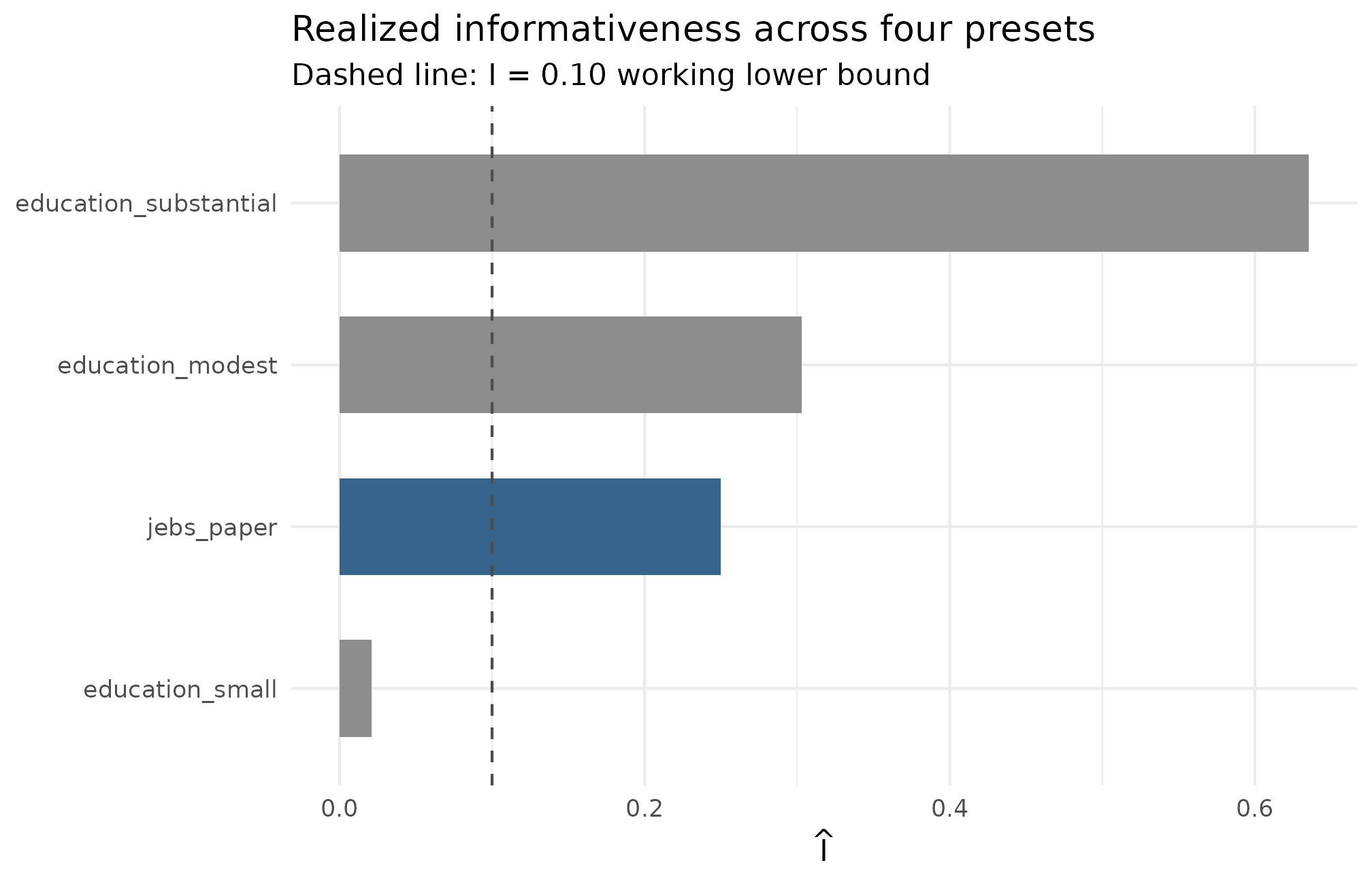

Realized informativeness across four site-size presets at seed = 1L. Each bar is one preset; the dashed reference line at I = 0.10 marks the practical lower bound below which empirical-Bayes estimates collapse toward the grand mean. The JEBS preset (I_hat = 0.250) sits comfortably above the line; the small-effects preset sits well below it — a calibration warning, not a bug, because its sigma_tau = 0.05 target is intentionally signal-poor.

Bars above the 0.10 line are healthy; bars below it mean partial pooling dominates regardless of analyst choice. The substantial-effects preset clears the line by the largest margin — $\sigma_\tau = 0.30$ pushes signal-to-noise up. The small-effects bar is small by design — that preset’s calibration warning made legible (Weiss et al., 2017), not a pathology.

3. Group B — did the dependence land where I asked?

realized_rank_corr() reads the residual-scale dependence (Spearman correlation of $z_j$ with $\widehat{se}_j^2$); the same function also accepts on = "marginal" to switch to the marginal-scale version, and realized_rank_corr_marginal() is a convenience alias for that case (Spearman of $\widehat\tau_j$ with $\widehat{se}_j^2$). Both take a multisitedgp_data object.

realized_rank_corr(dat)
#> [1] -0.1931161

realized_rank_corr_marginal(dat)
#> [1] -0.1931161

Both come in at $-0.193$. The JEBS preset declares rank_corr = 0, so the realized value is sampling noise around zero at $J = 50$ — well within the rule-of-thumb $\pm 0.20$ band the package treats as PASS. Values outside flip to WARN, and farther outside, to FAIL.

The two scales coincide here because the JEBS preset declares no covariate-induced effects in Layer 1: with no $X\beta$ shifting $\tau_j$, the marginal and residual ranks coincide. They diverge for designs with covariates; that divergence is what A4 · Covariates and precision dependence walks through end-to-end.

When Group B fires red — what to fix

First, confirm the declared dependence target on the printed multisitedgp_design object — the field is rank_corr (Layer 3). If the declared target is correct, verify the alignment method actually ran: the align_rank_corr() family couples $z_j$ to $\widehat{se}_j^2$ at the requested correlation. A non-zero declared target with a near-zero realized correlation means alignment was bypassed; a zero target with a far-from-zero realized correlation is sampling noise at the chosen $J$ — increase $J$ or accept the band. See A4 · Covariates and precision dependence for the alignment workflow and M4 · Precision dependence for the three injection methods.

Plot 2 — funnel view annotated with the dependence target

The funnel plot is the visual contract for Group B: standard error on the x-axis, observed estimate on the y-axis, and a roughly symmetric top-to-bottom scatter is the visual signature of $\rho_S = 0$.

plot_funnel(dat, caption = FALSE) +
  ggplot2::labs(
    title    = "Group B funnel — does dependence land at the target?",
    subtitle = "Symmetric cloud confirms rho_S target = 0 (realized -0.193, PASS)"
  )

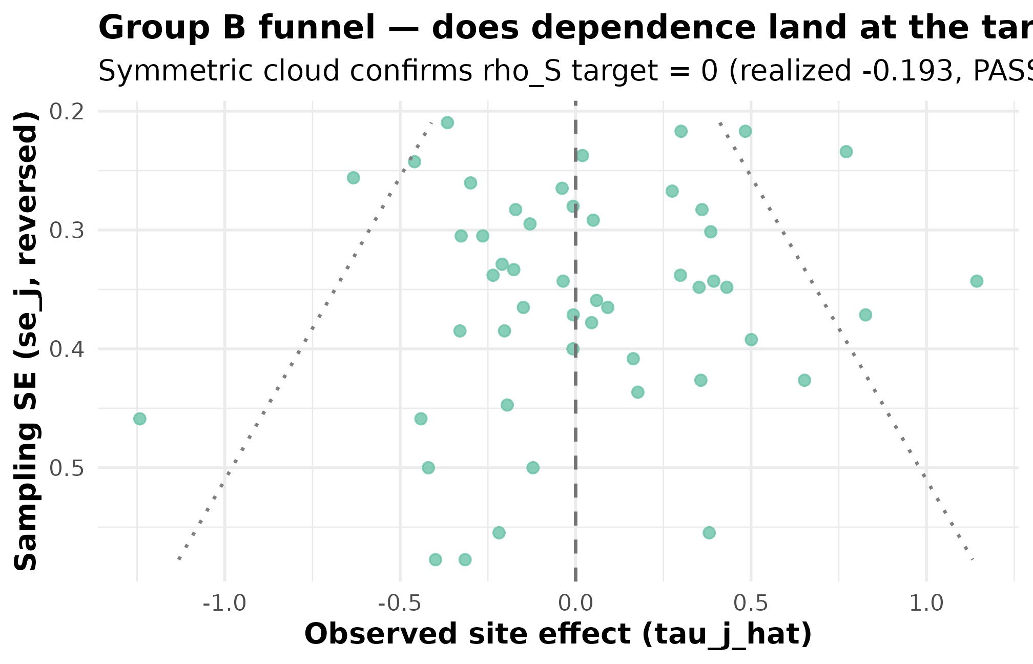
Funnel plot for preset_jebs_paper() at seed = 1L. Standard error on the x-axis (smaller = more precise); observed estimate on the y-axis. Symmetric scatter top-to-bottom across the precision range confirms rho_S target = 0; realized rank correlation -0.193 sits inside the ~0.20 PASS tolerance for J = 50. A FAIL would tilt the cloud — small-SE sites would skew toward one side of zero — and the rank-correlation status would flip.

Three things to read: top-to-bottom symmetry across the precision range is the PASS signature for $\rho_S = 0$. A tilt — small-SE sites piling up above zero with large-SE sites below (or vice versa) — is the visual FAIL. Cloud narrowing toward small SE is the site-size-driven signature; that is a Group A feature, read off Plot 1 and the $R$ scalar.

4. Group C — does the G shape look right?

ks_distance() is the Kolmogorov–Smirnov supremum distance between empirical CDFs; bhattacharyya_coef() is the histogram overlap coefficient. Both require a target sample y — Group C is the only group whose content depends on what the user is calibrating to, and there is no neutral default for “the right G shape.” Called without y, they error cleanly:

ks_distance(dat$z_j)
#> Error in `.abort_multisitedgp()`:
#> ✖ `y` must be a finite numeric vector.
#> ℹ `y` has length 0; minimum required length is 2.
#> → Pass finite numeric values for `y`.

For illustration, compare the JEBS mixture residuals to a Gaussian target sample. This is a deliberately mismatched reference: it shows how Group C reacts when the comparison distribution does not match the declared mixture shape. Reset the seed before drawing the target so the values below are reproducible across renders:

ks_distance(dat$z_j, y = y_target)
#> [1] 0.28

bhattacharyya_coef(dat$z_j, y = y_target)
#> [1] 0.6201199

Realized KS $\approx 0.28$ against ks_max = 0.10 and Bhattacharyya $\approx 0.62$ against bhattacharyya_min = 0.85. Both look like “failures” relative to the public gates, but the JEBS preset declares a mixture-shape latent rather than a Gaussian one — flagging a mixture against a Gaussian reference is the expected behavior, not a calibration error. The Group C row in summary(dat) carries the status target_source = "not_available" because the JEBS preset does not register a deterministic target G grid; in this regime the audit treats the row as reporting-only rather than a gate. The gates do fire as documented for designs that declare a Gaussian (or other deterministic-grid) target.

default_thresholds()[c("bhattacharyya_min", "ks_max")]
#> $bhattacharyya_min
#> [1] 0.85
#> 
#> $ks_max
#> [1] 0.1

When Group C fires red — what to fix

Group C FAIL on a working design (large $J$, large target sample) is a content-level mismatch between the declared G and the data being mimicked. Revisit the latent G choice and recalibrate against a real-data target through the workflow in A5 · Calibrating to real data. The G-distribution catalog lists the eight built-in shapes. At small $J$ a Group C FAIL is more often a power problem than a calibration problem; the quick check is to repeat the diagnostic at a synthetically larger $J$ and see whether the FAIL persists.

Plot 3 — Q-Q view of realized $z_j$ against Gaussian quantiles

For a Gaussian-G design, points line up on the 45-degree reference; for a mixture, heavy-tailed, or skewed design, the curve bends at the tails or the mode in a shape-specific way.

qq_df <- tibble::tibble(
  theoretical = qnorm(ppoints(length(dat$z_j))),
  empirical   = sort(dat$z_j)
)
ggplot2::ggplot(qq_df, ggplot2::aes(theoretical, empirical)) +
  ggplot2::geom_abline(slope = 1, intercept = 0,
                       linetype = "dashed", color = "grey45") +
  ggplot2::geom_point(size = 2.0, alpha = 0.78, color = "grey20") +
  ggplot2::labs(
    x = "Theoretical Gaussian quantile",
    y = expression(z[j] * " (sorted)"),
    title = "Q-Q plot: z_j vs Gaussian quantiles",
    subtitle = "Tail departures are the signature of the mixture latent"
  ) +
  ggplot2::theme_minimal(base_size = 11)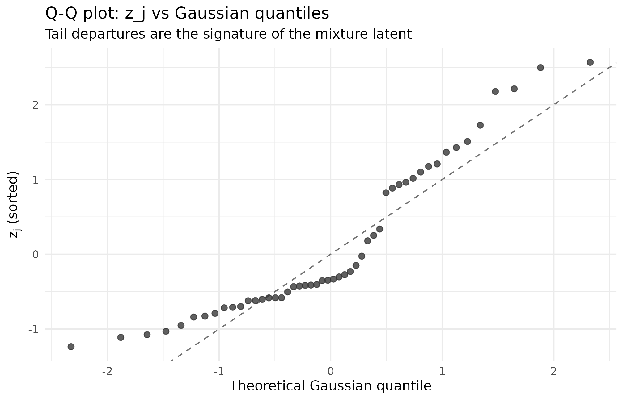

Q-Q plot of z_j (preset_jebs_paper, seed = 1L) against theoretical Gaussian quantiles. Departures from the 45-degree reference are the signature of the mixture shape; the central segment is approximately linear because the bulk of the latent is near-Gaussian, while the tails show the mixture’s lift. Read tail departures as the structural component of the KS distance from a Gaussian comparison.

Three things to read: linearity of the central segment (points near zero close to the 45-degree line means the bulk of the latent is near-Gaussian); tail-segment slope and curvature (S-shape signals heavier-than-Gaussian tails — a mixture or Student-t; a dog-leg signals a discrete component such as point-mass-and-slab); and sample-size noise at $J = 50$ (use this view in concert with the KS / Bhattacharyya numbers, not as a sole verdict).

5. Group D — will it work downstream?

mean_shrinkage() is the average shrinkage factor an empirical-Bayes estimator will apply (Walters, 2024); feasibility_index() is an effective-sample-size metric that gates whether partial pooling stabilizes at all.

mean_shrinkage(dat)
#> [1] 0.261965

feasibility_index(se2_j = dat$se2_j, sigma_tau = 0.2)
#> [1] 13.09825

Realized mean shrinkage is 0.262 — slightly below the canonical threshold mean_shrinkage_min = 0.30. This earns a WARN status: the design does enough partial-pooling work to benefit from a hierarchical estimator, but it is below the recommended floor. Feasibility index 13.1 — the Efron form, comfortably above the gate feasibility_min = 5.0. This is the equivalent of about 13 perfectly-informative sites’ worth of information after shrinkage. PASS.

Threshold band — written out

default_thresholds() returns five gates. The two that bear directly on Group D are mean_shrinkage_min and feasibility_min; the other three live with Groups A and C.

default_thresholds()
#> $mean_shrinkage_min
#> [1] 0.3
#> 
#> $feasibility_min
#> [1] 5
#> 
#> $R_max
#> [1] 30
#> 
#> $bhattacharyya_min
#> [1] 0.85
#> 
#> $ks_max
#> [1] 0.1

Gate	Group	Value	Direction	Meaning of FAIL/WARN
mean_shrinkage_min	D	0.30	floor	Partial pooling does too little work for a hierarchical estimator to add value.
feasibility_min	A/D	5.0	floor	Fewer than five sites’ worth of effective information after shrinkage.
R_max	A	30.0	ceiling	Ill-conditioned: a small subset of sites dominates the precision-weighted average.
bhattacharyya_min	C	0.85	floor	Realized G overlaps the target by less than 85 percent.
ks_max	C	0.10	ceiling	Worst-case CDF mismatch exceeds 10 percentage points.

To override a gate, edit the returned list and pass it to scenario_audit() via the thresholds argument:

th <- default_thresholds()
th$mean_shrinkage_min <- 0.25  # accept slightly lower S-bar
audit <- scenario_audit(grid, M = 50L, thresholds = th)

When Group D fires red — what to fix

To lift the feasibility index, raise $J$ or nj_mean. To lift mean shrinkage, raise $\sigma_\tau$ if the design plausibly supports it — partial pooling does more work when between-site variation is large relative to within-site noise. When both scalars sit far below threshold, reconsider whether partial pooling is the right tool at all: a fixed-effects estimator (no pooling) or a grand-mean estimator (full pooling) may be more honest than empirical Bayes.

Plot 4 — feasibility curve across average site size

The visual contract for Group D is a feasibility curve across average site size at fixed $\sigma_\tau$. As $\bar{n}_j$ grows, each site’s $\widehat{se}_j^2 \approx \kappa / \bar{n}_j$ shrinks, $S_j$ grows, and the feasibility index rises.

ggplot2::ggplot(groupD_df, ggplot2::aes(nj_mean, feasibility)) +
  ggplot2::geom_hline(yintercept = 5, linetype = "dashed", color = "grey45") +
  ggplot2::geom_line(linewidth = 0.9, color = "grey25") +
  ggplot2::geom_point(size = 2.6, color = "grey15") +
  ggplot2::geom_text(ggplot2::aes(label = sprintf("%.1f", feasibility)),
                     vjust = -0.9, size = 3.3) +
  ggplot2::labs(
    x = expression(bar(n)[j]),
    y = "Efron feasibility index",
    title = "Feasibility rises with average site size",
    subtitle = "preset_education_modest(), sigma_tau = 0.20; dashed line is the default gate (5.0)"
  ) +
  ggplot2::theme_minimal(base_size = 11)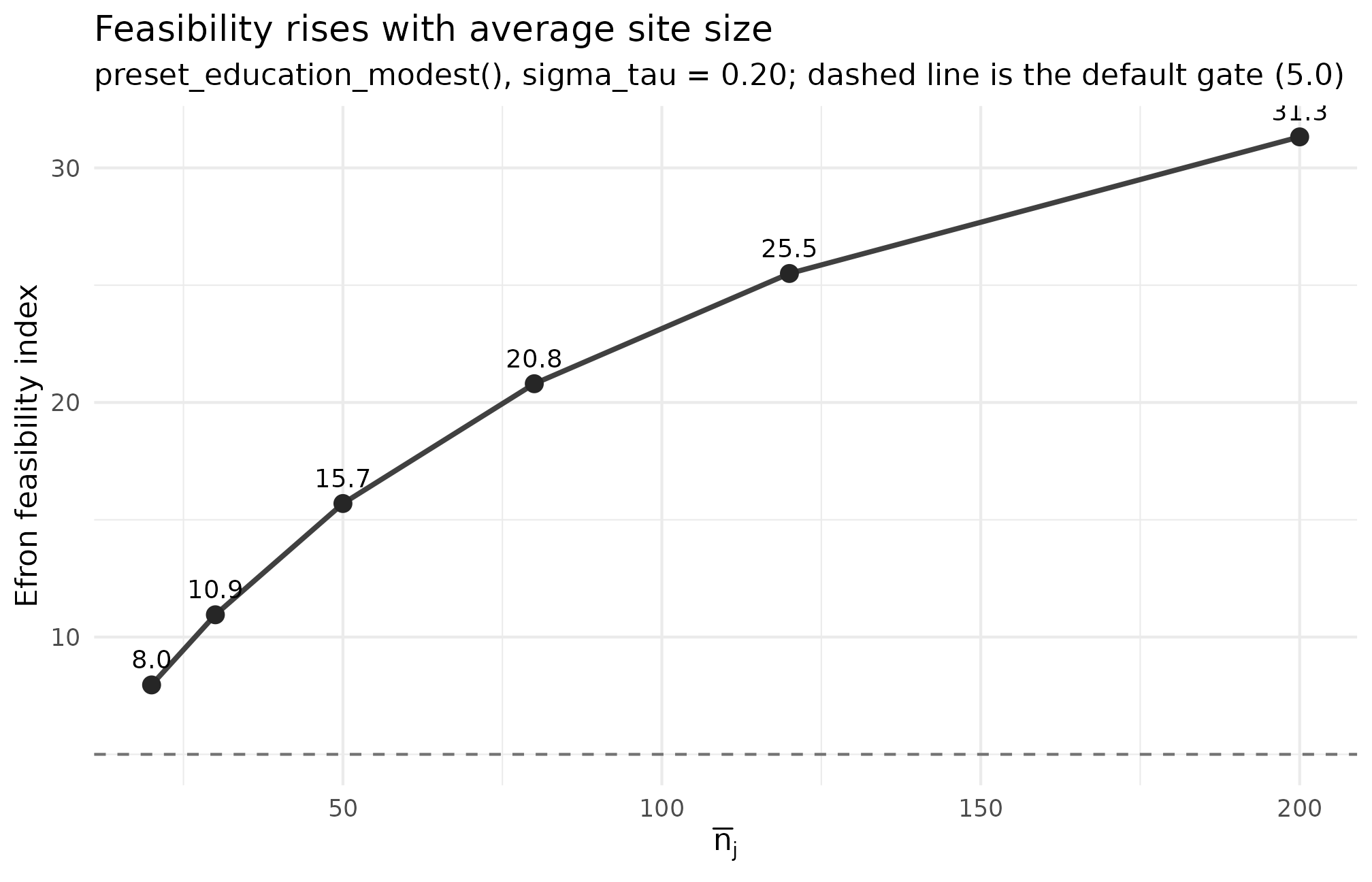

Efron feasibility index against average site size nj_mean (preset_education_modest, sigma_tau = 0.20, seed = 1L). The dashed reference at feasibility = 5 is the default lower gate; the curve grows because larger sites shrink each per-site SE and lift S_j toward 1. Use this curve to read the smallest defensible nj_mean for a target feasibility.

What to read: position relative to the dashed gate (above = clears, below = Group D FAIL); slope between adjacent points is the marginal feasibility you buy by adding 10 students per site (a flat slope at large $\bar{n}_j$ means diminishing returns — recruiting more sites buys more feasibility than enlarging existing ones); and where the curve crosses the gate is the minimum defensible average site size at this $\sigma_\tau$.

6. Triage workflow — what to do when a diagnostic fires red

The four sections above each end with a short “what to fix” rule. The card below collects all four. Paste it next to your simulation script or run it as the checklist on your next design review.

Group	What it asks	How to read	If FAIL — first move	Where the fix lives
A — scale	Did $I$ and $R$ hit their targets?	informativeness(dat), heterogeneity_ratio(dat$se2_j). Low $I$ (< 0.10), high $R$ (> 30).	Raise nj_mean (lifts $I$) or revisit $\sigma_\tau$. Narrow site sizes if $R$ excessive.	multisitedgp_design(); preset overrides.
B — dependence	Did rank correlation match the declared target?	realized_rank_corr(dat), realized_rank_corr_marginal(dat) vs. design rank_corr.	Verify Layer-3 alignment ran; confirm the declared target. Small $J$ widens the tolerance band.	align_rank_corr() family; A4; M4.
C — G shape	Does realized $z_j$ match the target G?	ks_distance(dat$z_j, y), bhattacharyya_coef(dat$z_j, y). Both REQUIRE y.	Calibrate against a real-data target; reconsider the latent G shape. Gate is power-bound at small $J$.	A5 · Calibrating to real data; M2 · G-distribution catalog.
D — feasibility	Will partial pooling work?	mean_shrinkage(dat), feasibility_index(dat$se2_j, sigma_tau) vs. default_thresholds().	Raise $J$ or nj_mean; reconsider the estimator if both sit deep below threshold.	feasibility_index(); estimator choice in A6.

Three reading rules. Answer Group A first — scale is the earliest design check and a Group A FAIL is almost always a design problem, not a downstream-tool problem. The Group B rule asks for the declared target, not the realized number — $-0.193$ against a declared $0$ is PASS at $J = 50$; the realized number alone is not actionable. The Group D rule has the longest fix list — lifting feasibility requires more sites, more data per site, or a different estimator, none of which is free (Walters, 2024).

7. Audit a grid before running the full study

A single working design is one row; a real simulation campaign covers a grid. design_grid() builds the factorial grid; scenario_audit() runs the four-question rubric on every cell with $M$ replicates and returns one summary row per cell. scenario_audit() requires its first argument to be a multisitedgp_design_grid (the output of design_grid()), not an arbitrary list of designs.

g <- design_grid(
  base_design = preset_education_modest(),
  J           = c(30L, 50L),
  sigma_tau   = c(0.15, 0.20),
  seed_root   = 12345L
)
g
#> # A tibble: 4 × 4
#>       J sigma_tau design                seed
#>   <int>     <dbl> <list>               <int>
#> 1    30      0.15 <mltstdg_ [29]>  948822067
#> 2    30      0.2  <mltstdg_ [29]> 1120920282
#> 3    50      0.15 <mltstdg_ [29]> 1960520344
#> 4    50      0.2  <mltstdg_ [29]> 1396277853

Four cells, one per $(J, \sigma_\tau)$ combination. The design list-column carries the per-cell multisitedgp_design, and seed carries a deterministic per-cell seed derived from seed_root. Now the audit at $M = 20$ replicates per cell:

audit <- scenario_audit(g, M = 20L)
audit[, c("cell_id", "J", "sigma_tau", "M",
          "status", "pass", "n_violations")]
#> # A tibble: 4 × 7
#>   cell_id     J sigma_tau     M status pass  n_violations
#>     <int> <int>     <dbl> <int> <chr>  <lgl>        <int>
#> 1       1    30      0.15    20 FAIL   FALSE            3
#> 2       2    30      0.2     20 FAIL   FALSE            2
#> 3       3    50      0.15    20 FAIL   FALSE            3
#> 4       4    50      0.2     20 FAIL   FALSE            2

scenario_audit() returns a tibble with 25 columns. The eight you reach for first:

• cell_id — integer 1, 2, …; matches the design_grid() printout.
• M — replicate count actually used; carries through so the audit is self-documenting.
• status — one-word verdict per cell: PASS / WARN / FAIL.
• pass — logical companion; TRUE only if no gate fired. Use it to filter the audit tibble.
• n_violations — count of distinct gates that fired. Three simultaneous gates point at where to look; one often resolves with a single override.
• fail_reasons — comma-separated names of gates at FAIL. The column to read when triaging a red cell — it points at which of the four groups broke.
• warn_reasons — same column for WARN-level gates.
• med_I_hat, q05_I_hat, q95_I_hat — median and 5/95 quantiles of realized $I$ across the cell’s $M$ replicates. The median is the headline; the bracket says how stable the median is.

The remaining 16 columns repeat the median/quantile pattern for $R$, mean shrinkage, the two flavors of feasibility, Bhattacharyya, and KS. Read them in groups of three, anchored on the medians:

audit[, c("cell_id", "J", "sigma_tau",
          "med_I_hat", "med_R_hat", "med_mean_shrinkage",
          "med_feasibility_efron", "fail_reasons")]
#> # A tibble: 4 × 8
#>   cell_id     J sigma_tau med_I_hat med_R_hat med_mean_shrinkage
#>     <int> <int>     <dbl>     <dbl>     <dbl>              <dbl>
#> 1       1    30      0.15     0.199      7.28              0.209
#> 2       2    30      0.2      0.309      8.12              0.318
#> 3       3    50      0.15     0.201      8.92              0.213
#> 4       4    50      0.2      0.302      9.86              0.313
#> # ℹ 2 more variables: med_feasibility_efron <dbl>, fail_reasons <chr>

Read down the fail_reasons column to see which gate is firing in each cell. The audit is honest about $M = 20$ being a smoke audit — the across-replicate medians stabilize as $M$ grows, and a cell that flags FAIL at $M = 20$ but clears at $M = 200$ is revealing sampling noise, not a structural failure of the design.

Recommended workflow

1. Build the grid with design_grid(..., seed_root = ...).
2. Run scenario_audit(grid, M = 50L) for a fast pre-check.
3. Drop or revise cells that fail the gates that matter for your study — Group A and D are usually the binding constraints; Group C binds only when the design declares a deterministic target G.
4. Run the full simulation only on the surviving cells.

For an end-to-end case study walking this workflow, see A6 · Case study — multisite trial. For wiring the audit’s hashes into a methods appendix, see Reproducibility and provenance.

8. Where to next

• A1 · Getting started and A2 · Choosing a preset — prior steps.
• A4 · Covariates and precision dependence — the Layer-3 alignment workflow that drives Group B.
• A5 · Calibrating to real data — the workflow when Group C fires on a real-data target.
• A6 · Case study — multisite trial — applies the §6 triage card to a realistic design grid.

For methodology, start with The two-stage DGP and read M2 / M3 / M4 in order.

References

The four-question rubric is introduced in Lee et al. (2025); the public thresholds in default_thresholds() are the package’s adaptation of the JEBS gates. Empirical-Bayes context for Group D is collected in Walters (2024). Education calibration anchors referenced in §2 are taken from Weiss et al. (2017).

Acknowledgments

This research was supported by the Institute of Education Sciences, U.S. Department of Education, through Grant R305D240078 to the University of Alabama. The opinions expressed are those of the authors and do not represent views of the Institute or the U.S. Department of Education.

Session info

#> R version 4.6.0 (2026-04-24)
#> Platform: x86_64-pc-linux-gnu
#> Running under: Ubuntu 24.04.4 LTS
#> 
#> Matrix products: default
#> BLAS:   /usr/lib/x86_64-linux-gnu/openblas-pthread/libblas.so.3 
#> LAPACK: /usr/lib/x86_64-linux-gnu/openblas-pthread/libopenblasp-r0.3.26.so;  LAPACK version 3.12.0
#> 
#> locale:
#>  [1] LC_CTYPE=C.UTF-8       LC_NUMERIC=C           LC_TIME=C.UTF-8       
#>  [4] LC_COLLATE=C.UTF-8     LC_MONETARY=C.UTF-8    LC_MESSAGES=C.UTF-8   
#>  [7] LC_PAPER=C.UTF-8       LC_NAME=C              LC_ADDRESS=C          
#> [10] LC_TELEPHONE=C         LC_MEASUREMENT=C.UTF-8 LC_IDENTIFICATION=C   
#> 
#> time zone: UTC
#> tzcode source: system (glibc)
#> 
#> attached base packages:
#> [1] stats     graphics  grDevices utils     datasets  methods   base     
#> 
#> other attached packages:
#> [1] ggplot2_4.0.3      multisiteDGP_0.1.1
#> 
#> loaded via a namespace (and not attached):
#>  [1] gtable_0.3.6       jsonlite_2.0.0     dplyr_1.2.1        compiler_4.6.0    
#>  [5] tidyselect_1.2.1   nleqslv_3.3.7      tidyr_1.3.2        jquerylib_0.1.4   
#>  [9] systemfonts_1.3.2  scales_1.4.0       textshaping_1.0.5  yaml_2.3.12       
#> [13] fastmap_1.2.0      R6_2.6.1           labeling_0.4.3     generics_0.1.4    
#> [17] knitr_1.51         tibble_3.3.1       desc_1.4.3         bslib_0.10.0      
#> [21] pillar_1.11.1      RColorBrewer_1.1-3 rlang_1.2.0        utf8_1.2.6        
#> [25] cachem_1.1.0       xfun_0.57          fs_2.1.0           sass_0.4.10       
#> [29] S7_0.2.2           cli_3.6.6          pkgdown_2.2.0      withr_3.0.2       
#> [33] magrittr_2.0.5     digest_0.6.39      grid_4.6.0         lifecycle_1.0.5   
#> [37] vctrs_0.7.3        evaluate_1.0.5     glue_1.8.1         farver_2.1.2      
#> [41] ragg_1.5.2         purrr_1.2.2        rmarkdown_2.31     tools_4.6.0       
#> [45] pkgconfig_2.0.3    htmltools_0.5.9

Lee, J., Che, J., Rabe-Hesketh, S., Feller, A., & Miratrix, L. (2025). Improving the estimation of site-specific effects and their distribution in multisite trials. Journal of Educational and Behavioral Statistics, 50(5), 731–764. https://doi.org/10.3102/10769986241254286

Walters, C. (2024). Empirical bayes methods in labor economics. In Handbook of labor economics (Vol. 5, pp. 183–260). Elsevier. https://doi.org/10.1016/bs.heslab.2024.11.001

Weiss, M. J., Bloom, H. S., Verbitsky-Savitz, N., Gupta, H., Vigil, A. E., & Cullinan, D. N. (2017). How much do the effects of education and training programs vary across sites? Evidence from past multisite randomized trials. Journal of Research on Educational Effectiveness, 10(4), 843–876. https://doi.org/10.1080/19345747.2017.1300719