M3 · Margin and SE models — site-size and direct-precision paths • multisiteDGP

Abstract

For methodologists choosing between a multisite-trial design (where per-site sample sizes determine sampling precision) and a meta-analytic design (where reported standard errors are the design surface), this vignette derives the two precision margins multisiteDGP exposes, contrasts the two front doors sim_multisite() and sim_meta(), demonstrates that the package enforces paradigm-strict dispatch by erroring on cross-door arguments, and shows the realized SE distribution under each path. You leave with the mapping rule for picking a path, two diagnostic plots (kappa-over-n overlay and (I, R)-implied target overlay), and the identifiability statement that lets the two paths be reasoned about independently.

1. Why two paradigms

Multisite trials and meta-analyses describe the same downstream quantity — a per-unit estimate $\hat\tau_j$ paired with a reported sampling standard error $\widehat{se}_j$ — but they hand the analyst a different design surface. A multisite-trial design arrives as a list of per-site sample sizes $n_j$ : the trialist negotiated a target enrolment with each site, the protocol fixed an allocation share $p$ between treatment and control, and the per-site sampling variance follows from $n_j$ via the closed-form $\widehat{se}_j^{\,2} = \kappa / n_j$ derived in M1: The two-stage DGP. A meta-analytic design, by contrast, arrives as a list of reported $(\hat\tau_j, \widehat{se}_j)$ pairs: studies in the corpus reported their effect sizes and standard errors directly, and the underlying per-study sample sizes are heterogeneous, sometimes unrecoverable, and in any case not the natural design knob a methodologist turns when asking “what happens to my estimator when the precision spread widens?”

multisiteDGP exposes both surfaces as separate front doors. The site-size-driven path (Paradigm A in the blueprint) takes per-site sample sizes — distributed via a truncated Gamma — and derives sampling variances. The direct-precision path (Paradigm B in the blueprint) takes informativeness and heterogeneity targets directly and constructs the SE marginal to match. Both paths route the same Layer 1 latent-effect generator, the same Layer 3 precision-dependence machinery, and the same Layer 4 observation draw; the only difference is Layer 2 — the SE-margin generator. Keeping the two paths separated at the front door — rather than rolling them into a single dispatcher — is what makes simulation provenance auditable: a reader can tell at a glance which design surface the simulation lives on, and the package errors on cross-door arguments before any compute happens.

2. Paradigm A — site-size-driven

2.1 The formal model

Under the site-size-driven path, the per-site sampling variance is the deterministic ratio of a configuration-derived constant $\kappa$ and the per-site sample size $n_j$ :

$\widehat{se}_j^{\,2} \;=\; \frac{\kappa}{n_j}, \qquad \kappa \;=\; \left(\frac{1}{p} + \frac{1}{1 - p}\right)(1 - R^2)\, s_Y^2.$

The closed form for $\kappa$ comes from the balanced-randomization Neyman variance: $p$ is the treatment-allocation share, $R^2$ is the share of outcome variance explained by site-level covariates (zero in the absence of covariates), and $s_Y^2$ is the residual outcome variance on the response scale. At the package defaults ( $p = 0.5$ , $R^2 = 0$ , $s_Y^2 = 1$ ), $\kappa = 4$ exactly. The per-site sample sizes are drawn from a truncated Gamma marginal with user-supplied conditional mean $\bar n_j$ , conditional CV $\mathrm{CV}$ , and lower truncation $n_{j,\min}$ :

$n_j \;\stackrel{\text{i.i.d.}}{\sim}\; \mathrm{TruncGamma}\bigl(\bar n_j,\, \mathrm{CV};\, n_{j,\min}\bigr).$

A two-line check confirms $\kappa$ at the defaults and the closed form under non-zero $R^2$ :

compute_kappa(p = 0.5, R2 = 0,   var_outcome = 1)
#> [1] 4
compute_kappa(p = 0.5, R2 = 0.4, var_outcome = 1)
#> [1] 2.4

The first call returns 4 (the JEBS default); the second returns $4 \cdot (1 - 0.4) = 2.4$ — covariate adjustment shrinks $\kappa$ multiplicatively. Section 5 returns to this with a kappa-rate overlay on a real simulation.

2.2 Two engines for the site-size margin

The truncated-Gamma marginal is implemented by two engines that hit two different invariants. Engine A1 (A1_legacy, legacy_jebs_censor_round) reproduces the JEBS paper’s published numerical results bit-for-bit: the engine matches the JEBS appendix’s exact RNG call sequence — rgamma(J) for site sizes, lower-censoring at $n_{j,\min}$ via pmax, integer rounding, then a row-shuffle inside dplyr::slice_sample(prop = 1) — and the canonical hash of its output under the published preset matches Lee et al. (2025)’s appendix output byte-for-byte. Engine A2 (A2_modern, trunc_gamma_moment) solves the truncated-Gamma moment equations numerically so that the conditional mean and CV given $n_j \ge n_{j,\min}$ exactly match the user-supplied $\bar n_j$ and $\mathrm{CV}$ . Engine A1’s censor-and-round procedure shifts those conditional moments away from the user inputs; Engine A2 keeps them on target. Both engines deliver the same closed-form $\widehat{se}_j^{\,2} = \kappa/n_j$ identity at the standardized residual scale — the package’s testable invariant T1b — and both feed the same downstream Layer 3 / Layer 4 machinery.

The choice is mechanical:

Pick engine = "A1_legacy" when the explicit goal is to reproduce Lee et al. (2025)’s published numerical results bit-for-bit (testable invariant T1a). The presets preset_jebs_paper() and preset_jebs_strict() wire this engine in by default.
Pick engine = "A2_modern" (the package default) for any new simulation. The conditional-moment match makes the user’s $(\bar n_j, \mathrm{CV})$ inputs faithful to the realized site-size distribution, which is the contract a methodologist running power studies, calibration sweeps, or sensitivity analyses needs.

2.3 The front door

The unified entry point for the site-size-driven path is sim_multisite(). Either pass a fully-constructed multisitedgp_design with paradigm = "site_size", or hand the wrapper flat arguments and the package builds the design inline:

dat_A <- sim_multisite(preset_education_modest(), seed = 1L)
dat_A
#> # A multisitedgp_data: 50 sites, paradigm = "site_size"
#> # Realized vs intended:
#> #   I: realized=0.303 (no target)
#> #   R: realized=10.167 (no target)
#> #   sigma_tau: target=0.200, realized=0.166, FAIL
#> #   rho_S: target=0.000, realized=0.254, PASS
#> #   rho_S_marg: realized=0.254 (no target)
#> #   Feasibility: WARN (n_eff=15.693)
#> # A tibble: 50 × 7
#>   site_index    z_j   tau_j tau_j_hat  se_j  se2_j   n_j
#>        <int>  <dbl>   <dbl>     <dbl> <dbl>  <dbl> <int>
#> 1          1 -0.626 -0.125    -0.329  0.329 0.108     37
#> 2          2  0.184  0.0367    0.0481 0.270 0.0727    55
#> 3          3 -0.836 -0.167    -0.399  0.254 0.0645    62
#> 4          4  1.60   0.319     0.410  0.577 0.333     12
#> 5          5  0.330  0.0659   -0.146  0.324 0.105     38
#> 6          6 -0.820 -0.164     0.265  0.243 0.0588    68
#> # ℹ 44 more rows
#> # Use summary(df) for the full diagnostic report.

The print method’s diagnostic block reports the realized informativeness I near 0.30, the realized heterogeneity ratio R above 10, and the kappa-rate identity $\widehat{se}_j^{\,2} \cdot n_j = \kappa = 4$ holding by construction:

range(dat_A$se2_j * dat_A$n_j)
#> [1] 4 4
unique(round(dat_A$se2_j * dat_A$n_j, 8))
#> [1] 4

The range() check returns (4, 4) and the unique() check returns the single value 4 — the kappa-rate identity holds for every site, the testable invariant T3 in M1 §7. The realized informativeness reads back via either the diagnostics attribute or the standalone helper:

attr(dat_A, "diagnostics")$I_hat
#> [1] 0.3028032
compute_I(dat_A$se2_j, sigma_tau = 0.20)
#> [1] 0.3028032

Both calls return the same value (0.303) — the diagnostic block stores the result of a compute_I() call on the realized sampling variances, and the standalone helper recomputes it from the same vector. The realized $I$ falls below the design intent slightly because the kappa-over- $n_j$ marginal carries Jensen gap from the $n_j$ heterogeneity (CV = 0.5).

2.4 When to pick this path

The site-size-driven path fits the design surface when (a) the study specifies per-site sample sizes — so $\bar n_j$ , $\mathrm{CV}$ , and $n_{j,\min}$ are quantities you can defend on substantive grounds — and (b) the precision heterogeneity that emerges from the site-size distribution is itself part of the simulation question. Power calculations for actual multisite trials, calibration sweeps against realized sample-size distributions in the Weiss et al. (2017) education-trial benchmarks, and any JEBS-paper reproduction (Lee et al., 2025) all fit here. The path’s stochasticity — the realized $(I, R)$ are consequences of the $(\bar n_j, \mathrm{CV})$ draws, not exact inputs — is the feature, not the bug: it makes the simulation faithful to the trial specification rather than to a post-hoc precision target.

The Layer 2 generator is exposed individually as gen_site_sizes() for users composing the four layers manually.

3. Paradigm B — direct-precision

3.1 The formal model

Under the direct-precision path, the user supplies the two precision diagnostics directly: the mean informativeness scalar $I$ and the heterogeneity ratio $R$ . The Layer 2 generator back-calculates a deterministic SE marginal that hits both targets exactly. The informativeness identity from (Lee et al., 2025)’s Equation (4) implies that the geometric mean of $\widehat{se}_j^{\,2}$ is determined by $\sigma_\tau$ and $I$ :

$\mathrm{GM}\bigl(\widehat{se}_j^{\,2}\bigr) \;=\; \sigma_\tau^{\,2} \cdot \frac{1 - I}{I}.$

The heterogeneity ratio fixes the spread around the geometric mean. The package’s grid construction places the $J$ values log-evenly over the interval $[\mathrm{GM} \cdot R^{-1/2}, \mathrm{GM} \cdot R^{1/2}]$ :

$\widehat{se}_j^{\,2} \;=\; \mathrm{GM} \cdot R^{(j-1)/(J-1) - 1/2}, \qquad j = 1, \ldots, J.$

The construction is the Yu-Zhang-style log-even spacing (Yu & Zhang (2005)’s quantile parameterization in spirit, applied here to the SE marginal rather than the latent-effect shape). The endpoint arithmetic guarantees that the multiset’s geometric mean is $\mathrm{GM}$ exactly and its max-over-min ratio is $R$ exactly. The construction is deterministic: no randomness enters the SE marginal itself, only the optional shuffle = TRUE permutation of the grid values across sites. The site-size column $n_j$ is NA_integer_ — this path discards the per-site sample size entirely.

3.2 The front door

The unified entry point for the direct-precision path is sim_meta(). The minimal call passes flat $(J, I, R, \sigma_\tau)$ arguments and lets the wrapper build the direct-paradigm design inline:

dat_B <- sim_meta(J = 50L, I = 0.30, R = 2, sigma_tau = 0.20, seed = 1L)
dat_B
#> # A multisitedgp_meta: 50 sites, paradigm = "direct"
#> # Realized vs intended:
#> #   I: target=0.300, realized=0.300, PASS
#> #   R: target=2.000, realized=2.000, PASS
#> #   sigma_tau: target=0.200, realized=0.166, FAIL
#> #   rho_S: target=0.000, realized=-0.093, PASS
#> #   rho_S_marg: realized=-0.093 (no target)
#> #   Feasibility: WARN (n_eff=15.087)
#> # A tibble: 50 × 7
#>   site_index    z_j   tau_j tau_j_hat  se_j  se2_j   n_j
#>        <int>  <dbl>   <dbl>     <dbl> <dbl>  <dbl> <int>
#> 1          1 -0.626 -0.125    -0.0218 0.311 0.0967    NA
#> 2          2  0.184  0.0367    0.407  0.348 0.121     NA
#> 3          3 -0.836 -0.167    -0.276  0.358 0.128     NA
#> 4          4  1.60   0.319     0.438  0.322 0.104     NA
#> 5          5  0.330  0.0659    0.160  0.351 0.123     NA
#> 6          6 -0.820 -0.164    -0.325  0.296 0.0876    NA
#> # ℹ 44 more rows
#> # Use summary(df) for the full diagnostic report.

The print method’s diagnostic block confirms the (I, R) targets are hit exactly: I: target = 0.300, realized = 0.300, PASS and R: target = 2.000, realized = 2.000, PASS. The n_j column is NA across all 50 rows — the direct-precision path has no site-size margin to populate.

The exactness is verifiable via the diagnostics attribute, which under this path adds target_I, target_R, I_error, R_error, I_exact, and R_exact slots:

diag_B <- attr(dat_B, "diagnostics")
c(I_hat = diag_B$I_hat, target_I = diag_B$target_I,
  I_error = diag_B$I_error, I_exact = diag_B$I_exact)
#>    I_hat target_I  I_error  I_exact 
#>      0.3      0.3      0.0      1.0
c(R_hat = diag_B$R_hat, target_R = diag_B$target_R,
  R_error = diag_B$R_error, R_exact = diag_B$R_exact)
#>    R_hat target_R  R_error  R_exact 
#>        2        2        0        1

Both error slots are zero, both exactness flags are TRUE. The underlying Layer 2 generator is exposed individually as gen_se_direct() for manual composition.

3.3 When to pick this path

The direct-precision path fits the design surface when (a) the study specifies (or the methodologist controls) the precision diagnostics themselves rather than a sample-size distribution — meta-analyses where the corpus reports $(\hat\tau_j, \widehat{se}_j)$ without recoverable $n_j$ , Fay-Herriot small-area estimation problems, or methods-comparison studies that need to fix informativeness exactly across cells of a sweep — and (b) the methodologist wants the realized $(I, R)$ to match the targets bit-for-bit, not stochastically. The deterministic-grid construction is the feature: when comparing a shrinkage estimator across $I \in \{0.10, 0.30, 0.50, 0.80\}$ , the direct-precision path lets the methodologist hold the precision-side design constant and isolate estimator behavior, free from the sample-size noise the site-size-driven path introduces by design.

Two presets wire the direct-precision path in by default: preset_meta_modest() for modest meta-analytic informativeness and preset_small_area_estimation() for the wider precision spread typical of small-area surveys. The canonical applied walkthrough is A7: Case study — meta-analysis.

4. The two paradigms as a contract table

The four-column contract below is the operational summary: which formal model each path fixes at Layer 2, when to reach for it, and which front door to call. Cross-door arguments are rejected by both wrappers (Section 6 demonstrates).

Paradigm	Formal model (Layer 2 SE margin)	When to pick	Front door / preset family
Site-size-driven (Paradigm A)	$\widehat{se}_j^{\,2} = \kappa / n_j$ with $\kappa = (1/p + 1/(1-p))(1 - R^2) s_Y^2$ and $n_j \sim \mathrm{TruncGamma}(\bar n_j, \mathrm{CV}; n_{j,\min})$	Per-site sample sizes are part of the design surface; precision heterogeneity is a consequence of the site-size distribution.	`sim_multisite()`; `preset_jebs_paper()`, `preset_jebs_strict()`, `preset_education_modest()`, `preset_education_substantial()`, `preset_education_small()`, `preset_walters_2024()`, `preset_twin_towers()`
Direct-precision (Paradigm B)	$\widehat{se}_j^{\,2} = \mathrm{GM} \cdot R^{(j-1)/(J-1) - 1/2}$ with $\mathrm{GM} = \sigma_\tau^{\,2}(1 - I)/I$ , $n_j = \mathtt{NA\_integer\_}$	Precision diagnostics $(I, R)$ are part of the design surface; per-site sample sizes are absent or incidental.	`sim_meta()`; `preset_meta_modest()`, `preset_small_area_estimation()`

The two paths are isomorphic at the level of the realized $\widehat{se}_j^{\,2}$ vector — once Layer 2 has populated se2_j, Layer 3 and Layer 4 see the same input and run identically. This is what makes the contrast a front-door distinction rather than a downstream one: the design surface differs, but the simulation pipeline downstream of Layer 2 is shared.

5. The realized SE distribution under each paradigm

The two plots below are diagnostic, not decorative: each one shows the realized SE marginal under one path and overlays the formal-model target the path was supposed to hit. Read each plot for whether the realized distribution lands on the target overlay.

5.1 Plot 1 — Paradigm A realized SE distribution

Under the site-size-driven path with preset_education_modest(), the SE marginal inherits the right-skew of the truncated-Gamma site- size marginal: small- $n_j$ sites correspond to large- $\widehat{se}_j$ sites. The overlay shows the deterministic curve $\kappa/n_j$ at $\kappa = 4$ across the realized $n_j$ range — every realized point sits exactly on the curve, not approximately, because the kappa-rate identity is deterministic at the package’s testable invariant T3.

set.seed(1L)
dat_A <- sim_multisite(preset_education_modest(), seed = 1L)
kappa_A <- compute_kappa(p = 0.5, R2 = 0, var_outcome = 1)
df_A <- tibble::tibble(
  n_j   = dat_A$n_j,
  se2_j = dat_A$se2_j
)
n_grid <- seq(min(df_A$n_j), max(df_A$n_j), length.out = 200)
df_curve <- tibble::tibble(
  n_j      = n_grid,
  se2_curve = kappa_A / n_grid
)

p_top <- ggplot(df_A, aes(x = se2_j)) +
  geom_histogram(bins = 18, fill = "#1B4965", colour = "white", alpha = 0.85) +
  labs(x = NULL, y = "count") +
  theme_minimal(base_size = 9) +
  theme(panel.grid.minor = element_blank(),
        axis.text.x = element_blank(), axis.ticks.x = element_blank())

p_bottom <- ggplot(df_A, aes(x = n_j, y = se2_j)) +
  geom_line(data = df_curve, aes(x = n_j, y = se2_curve),
            colour = "grey40", linewidth = 0.6) +
  geom_point(alpha = 0.85, size = 2, colour = "#1B4965") +
  labs(
    x = expression(n[j]~"  (per-site sample size)"),
    y = expression(widehat(se)[j]^{2}~"  (sampling variance)")
  ) +
  theme_minimal(base_size = 11) +
  theme(panel.grid.minor = element_blank())

# Compose without depending on patchwork (soft dep).
gridExtra::grid.arrange(
  p_top,
  p_bottom,
  ncol = 1, heights = c(1, 4)
)

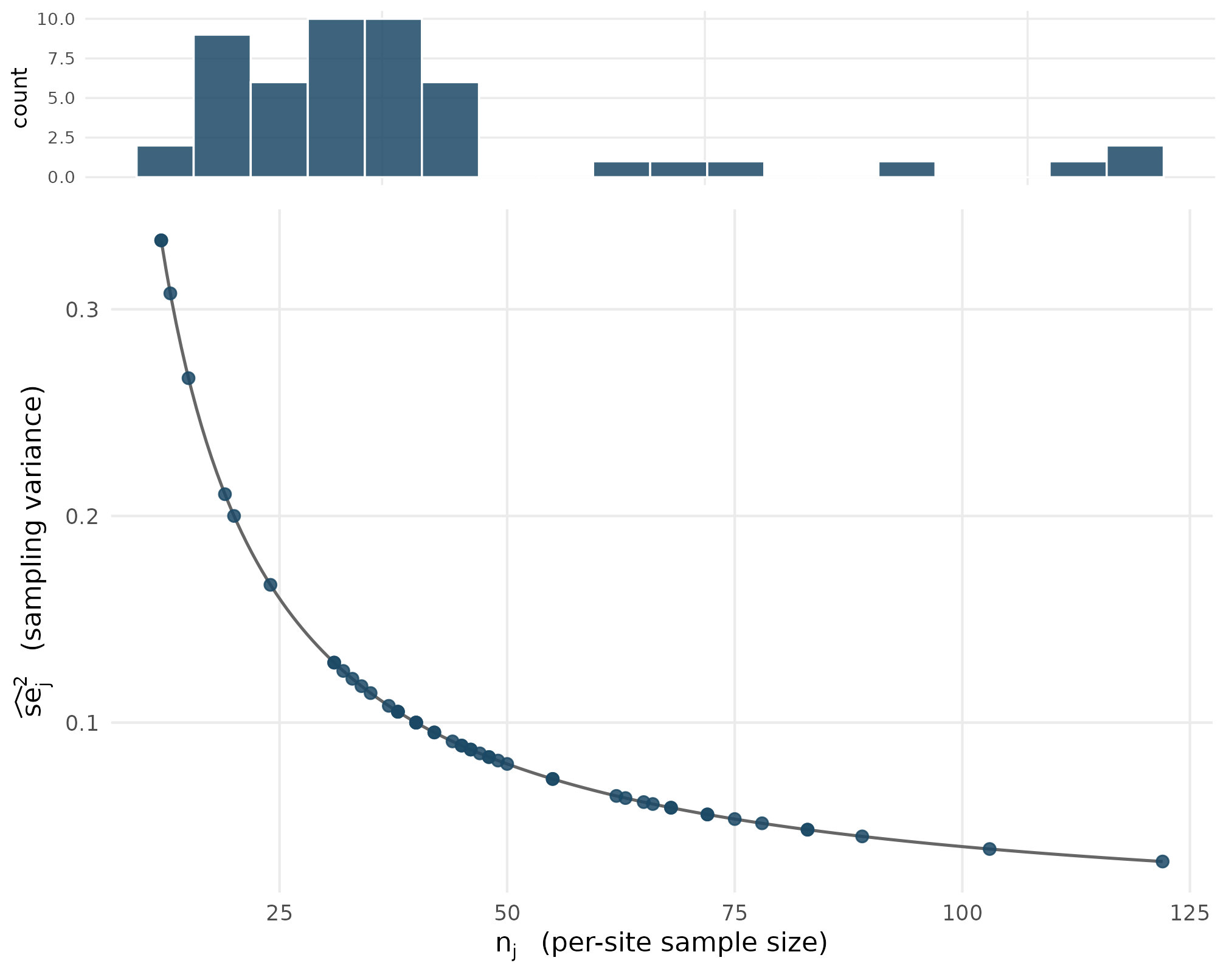
Two-panel composite figure showing a histogram of se squared values on top and a scatter of se squared against n_j with a kappa-over-n curve overlaid below. Realized points sit exactly on the curve.

Paradigm A realized se squared values from preset_education_modest at J = 50 (filled dots) sit exactly on the kappa-over-n curve (solid line, kappa = 4). The histogram on the upper margin shows the right-skewed se squared distribution that emerges from the truncated-Gamma site-size marginal. Confirms the kappa-rate identity (T3) and the right-skew shape consequence of n_j heterogeneity at CV = 0.5.

The single curve in the lower panel is the closed-form $\widehat{se}_j^{\,2} = \kappa/n_j$ at $\kappa = 4$ . Every realized point sits on the curve to floating-point precision (not approximately) because the kappa-rate identity is deterministic at Layer 2 — there is no Layer-2 noise on top of the closed form. The upper-panel histogram is the marginal of $\widehat{se}_j^{\,2}$ realized at $J = 50$ : the right tail at large $\widehat{se}_j^{\,2}$ comes from the small- $n_j$ tail of the truncated-Gamma site-size marginal, and the bulk near $\widehat{se}_j^{\,2} \approx 0.07$ comes from the centre of mass at $n_j \approx 50$ . The kappa-over- $n$ curve and the realized distribution carry exactly the same information — the right-skew is the sole consequence of the truncated-Gamma right-skew.

5.2 Plot 2 — Paradigm B realized SE distribution

Under the direct-precision path with $J = 50$ , $I = 0.30$ , $R = 2$ , $\sigma_\tau = 0.20$ , the SE marginal is the deterministic log-even grid. The overlay shows the implied geometric mean $\mathrm{GM} = \sigma_\tau^{\,2}(1 - I)/I = 0.0933$ as a vertical line and the implied min/max boundaries $\mathrm{GM} \cdot R^{\pm 1/2}$ as two further vertical lines. Every realized $\widehat{se}_j^{\,2}$ falls inside the $[\mathrm{GM}/\sqrt{R}, \mathrm{GM}\sqrt{R}]$ interval, the multiset’s geometric mean lands on the central line, and the multiset’s max-over-min ratio equals $R$ exactly.

set.seed(1L)
dat_B <- sim_meta(J = 50L, I = 0.30, R = 2, sigma_tau = 0.20, seed = 1L)
sigma_tau_B <- 0.20
I_B <- 0.30
R_B <- 2
GM_target <- sigma_tau_B^2 * (1 - I_B) / I_B
df_B <- tibble::tibble(se2_j = dat_B$se2_j)
GM_realized <- exp(mean(log(df_B$se2_j)))
range_B <- range(df_B$se2_j)

GM_target
#> [1] 0.09333333
GM_realized
#> [1] 0.09333333
range_B
#> [1] 0.06599663 0.13199327
range_B[2] / range_B[1]
#> [1] 2

The realized geometric mean equals the target $0.0933$ to floating- point precision; the realized range $[0.0660, 0.1320]$ lands on $[\mathrm{GM}/\sqrt{2}, \mathrm{GM}\sqrt{2}]$ exactly; the max-over-min ratio is 2, the requested $R$ .

ggplot(df_B, aes(x = se2_j)) +
  geom_histogram(bins = 18, fill = "#62929E", colour = "white", alpha = 0.85) +
  geom_vline(xintercept = GM_target, colour = "#1B4965",
             linewidth = 0.7) +
  geom_vline(xintercept = GM_target / sqrt(R_B), linetype = "dashed",
             colour = "grey40") +
  geom_vline(xintercept = GM_target * sqrt(R_B), linetype = "dashed",
             colour = "grey40") +
  annotate("text", x = GM_target, y = Inf, vjust = 1.4,
           label = "GM target", colour = "#1B4965", size = 3.2) +
  annotate("text", x = GM_target / sqrt(R_B), y = Inf, vjust = 1.4,
           label = "GM / sqrt(R)", colour = "grey30", size = 3.0) +
  annotate("text", x = GM_target * sqrt(R_B), y = Inf, vjust = 1.4,
           label = "GM * sqrt(R)", colour = "grey30", size = 3.0) +
  labs(
    x        = expression(widehat(se)[j]^{2}~"  (sampling variance)"),
    y        = "count",
    title    = "Paradigm B — direct-precision SE marginal at J = 50",
    subtitle = "I = 0.30, R = 2, sigma_tau = 0.20  ->  GM = 0.0933, range = [0.0660, 0.1320]"
  ) +
  theme_minimal(base_size = 11) +
  theme(panel.grid.minor = element_blank())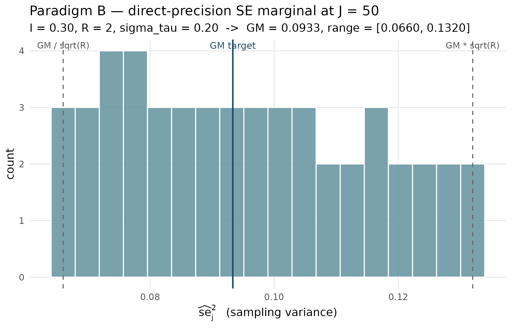

Histogram of se squared values from a Paradigm B simulation. A vertical line marks the geometric mean target; two dashed vertical lines mark the implied min and max. Histogram bars span exactly between the dashed lines.

Paradigm B realized se squared values from sim_meta(J = 50, I = 0.30, R = 2, sigma_tau = 0.20) (histogram). Vertical solid line: implied geometric mean GM = sigma_tau squared times (1 - I) over I = 0.0933. Dashed lines: GM divided by square root of R and GM times square root of R, the implied min and max. Confirms the deterministic grid hits the (I, R)-implied target exactly: every realized point lies inside the bracket, GM is on the solid line, and max over min equals 2.

Three things to read off the figure. First, the histogram is bounded exactly by the two dashed vertical lines — the $J = 50$ realized $\widehat{se}_j^{\,2}$ values fall inside $[\mathrm{GM}/\sqrt{R}, \mathrm{GM}\sqrt{R}]$ by construction, with the endpoints attained at $j = 1$ and $j = J$ . Second, the histogram’s shape is approximately uniform on the log scale (the design choice was log-even spacing) — the visible mild non-uniformity in linear bins reflects the log-to-linear stretch, not a design failure. Third, the solid central line at $\mathrm{GM} = 0.0933$ sits exactly at the geometric centre of the multiset.

The contrast between the two plots is exactly the contrast between the two paradigms: the site-size-driven path produces an SE distribution whose shape is a consequence of the site-size choice (right-skewed, with a long tail from small- $n_j$ sites); the direct-precision path produces an SE distribution whose shape is specified (a log-even grid bounded by the (I, R) target).

6. Identifiability and switching

The two paradigms share the same Layer 2 output signature — se2_j, se_j, and an n_j column populated under Paradigm A and NA_integer_ under Paradigm B — but their input signatures are disjoint. Paradigm A consumes $(\bar n_j, \mathrm{CV}, n_{j,\min}, p, R^2, s_Y^2, \mathrm{engine})$ ; Paradigm B consumes $(I, R, \mathrm{shuffle}, \mathrm{se\_fn}, \mathrm{se\_args})$ . The package keeps the two input vocabularies separated at the front door: handing sim_meta() a Paradigm A argument or sim_multisite() a Paradigm B argument is rejected with a coherence error before any compute happens.

sim_meta(J = 50L, nj_mean = 80, cv = 0.5, sigma_tau = 0.20, seed = 1L)
#> Error in `.abort_multisitedgp()`:
#> ✖ `sim_meta()` received site-size argument(s).
#> ℹ Wrong-door argument(s): nj_mean, cv.
#> → Use `sim_multisite()` for site-size designs or remove those arguments.

The error message names the wrong-door arguments (nj_mean, cv) and points to the correct front door (sim_multisite()). The same coherence check runs on the sister wrapper:

sim_multisite(J = 50L, I = 0.30, R = 2, sigma_tau = 0.20, seed = 1L)
#> Error in `.abort_multisitedgp()`:
#> ✖ `sim_multisite()` received direct meta-analysis argument(s).
#> ℹ Wrong-door argument(s): I, R.
#> → Use `sim_meta()` for `(I, R)` or direct-SE designs.

Again, the wrong-door arguments (I, R) are named and the caller is redirected to sim_meta(). The construction-time check is deliberate: cross-paradigm dispatch is strict by design, so the provenance attribute on a returned object always reflects exactly one paradigm and never an implicit mix. A simulation labelled paradigm = "site_size" in the diagnostics block was generated by the site-size-driven Layer 2 generator, not by Paradigm B with post-hoc relabelling.

The same paradigm-strict contract holds at the multisitedgp_design() level. Constructing a design with paradigm = "site_size" and then handing it to sim_meta() — or constructing a design with paradigm = "direct" and handing it to sim_multisite() — is also rejected. The wrapper checks design$paradigm against its own locked paradigm at entry. Below, an explicit Paradigm A design is forced through sim_meta():

des_A <- multisitedgp_design(
  paradigm = "site_size",
  J        = 50L,
  sigma_tau = 0.20,
  nj_mean  = 50,
  cv       = 0.50,
  nj_min   = 10L
)
sim_meta(des_A, seed = 1L)
#> Error in `.abort_multisitedgp()`:
#> ✖ `sim_meta()` requires `paradigm = "direct"`.
#> ℹ Got `design$paradigm = "site_size"`.
#> → Use `sim_multisite()` for site-size designs.

The error message names the design’s paradigm ("site_size") and points to the correct sister wrapper. The package never silently re-labels a design; it always errors and lets the caller decide.

Why this matters. A simulation pipeline that conflates the two paradigms — for example, by dispatching on a flag and silently swapping the Layer 2 generator — would let provenance drift on re-run: the same code path could yield different attr(x, "diagnostics")$paradigm values depending on argument order. The paradigm-strict front door rules that drift out at construction time. This is the operational form of the M1 §4 four-layer factorization: Layer 2 is the only differentiating layer between the two paths, so keeping the two front doors disjoint is the cleanest place to draw the line.

The single point where the two paths can be reasoned about jointly is the realized informativeness scalar $I$ . Under Paradigm A, $I$ is a consequence of $(\bar n_j, \mathrm{CV})$ via the Jensen gap on $\kappa/n_j$ ; under Paradigm B, $I$ is an input. The helper compute_I() reads the realized $I$ from any se2_j vector regardless of which path generated it:

compute_I(dat_A$se2_j, sigma_tau = 0.20)
#> [1] 0.3028032
compute_I(dat_B$se2_j, sigma_tau = 0.20)
#> [1] 0.3

The Paradigm A simulation lands at $I \approx 0.303$ and the Paradigm B simulation at exactly $0.300$ — the diagnostic helper itself is paradigm-blind, but the simulations it reads are paradigm-strict at the front door.

7. Where to next

A1: Getting started — applied walkthrough of the site-size-driven path from preset to diagnostics.
A6: Case study — multisite trial — full Paradigm A workflow including precision dependence and shrinkage diagnostics.
A7: Case study — meta-analysis — full Paradigm B workflow, including handoff to metafor via as_metafor().
M1: The two-stage DGP — the formal factorization; this vignette zoomed in on Layer 2 and how the two Layer-2 generators differ.
M4: Precision dependence theory — the rank, copula, and hybrid alignment methods that sit on top of Layer 2 in both paradigms.

References

The site-size-driven path’s $\kappa$ closed form and Engine A1’s bit-identical reproducibility contract come from Lee et al. (2025). The empirical-Bayes context for treating reported sampling standard errors as known — relevant to both paths but especially to the direct-precision path’s plug-in of $(\hat\tau_j, \widehat{se}_j)$ pairs from a meta-analytic corpus — is collected in Walters (2024). The education-trial calibration heritage that motivates the preset_education_modest() and sister Paradigm A presets is from Weiss et al. (2017).

Acknowledgments

This research was supported by the Institute of Education Sciences, U.S. Department of Education, through Grant R305D240078 to the University of Alabama. The opinions expressed are those of the authors and do not represent views of the Institute or the U.S. Department of Education.

Session info

#> R version 4.6.0 (2026-04-24)
#> Platform: x86_64-pc-linux-gnu
#> Running under: Ubuntu 24.04.4 LTS
#> 
#> Matrix products: default
#> BLAS:   /usr/lib/x86_64-linux-gnu/openblas-pthread/libblas.so.3 
#> LAPACK: /usr/lib/x86_64-linux-gnu/openblas-pthread/libopenblasp-r0.3.26.so;  LAPACK version 3.12.0
#> 
#> locale:
#>  [1] LC_CTYPE=C.UTF-8       LC_NUMERIC=C           LC_TIME=C.UTF-8       
#>  [4] LC_COLLATE=C.UTF-8     LC_MONETARY=C.UTF-8    LC_MESSAGES=C.UTF-8   
#>  [7] LC_PAPER=C.UTF-8       LC_NAME=C              LC_ADDRESS=C          
#> [10] LC_TELEPHONE=C         LC_MEASUREMENT=C.UTF-8 LC_IDENTIFICATION=C   
#> 
#> time zone: UTC
#> tzcode source: system (glibc)
#> 
#> attached base packages:
#> [1] stats     graphics  grDevices utils     datasets  methods   base     
#> 
#> other attached packages:
#> [1] ggplot2_4.0.3      multisiteDGP_0.1.1
#> 
#> loaded via a namespace (and not attached):
#>  [1] gtable_0.3.6       jsonlite_2.0.0     dplyr_1.2.1        compiler_4.6.0    
#>  [5] tidyselect_1.2.1   nleqslv_3.3.7      gridExtra_2.3      jquerylib_0.1.4   
#>  [9] systemfonts_1.3.2  scales_1.4.0       textshaping_1.0.5  yaml_2.3.12       
#> [13] fastmap_1.2.0      R6_2.6.1           labeling_0.4.3     generics_0.1.4    
#> [17] knitr_1.51         tibble_3.3.1       desc_1.4.3         bslib_0.10.0      
#> [21] pillar_1.11.1      RColorBrewer_1.1-3 rlang_1.2.0        cachem_1.1.0      
#> [25] xfun_0.57          fs_2.1.0           sass_0.4.10        S7_0.2.2          
#> [29] cli_3.6.6          pkgdown_2.2.0      withr_3.0.2        magrittr_2.0.5    
#> [33] digest_0.6.39      grid_4.6.0         lifecycle_1.0.5    vctrs_0.7.3       
#> [37] evaluate_1.0.5     glue_1.8.1         farver_2.1.2       ragg_1.5.2        
#> [41] rmarkdown_2.31     tools_4.6.0        pkgconfig_2.0.3    htmltools_0.5.9

Lee, J., Che, J., Rabe-Hesketh, S., Feller, A., & Miratrix, L. (2025). Improving the estimation of site-specific effects and their distribution in multisite trials. Journal of Educational and Behavioral Statistics, 50(5), 731–764. https://doi.org/10.3102/10769986241254286

Walters, C. (2024). Empirical bayes methods in labor economics. In Handbook of labor economics (Vol. 5, pp. 183–260). Elsevier. https://doi.org/10.1016/bs.heslab.2024.11.001

Weiss, M. J., Bloom, H. S., Verbitsky-Savitz, N., Gupta, H., Vigil, A. E., & Cullinan, D. N. (2017). How much do the effects of education and training programs vary across sites? Evidence from past multisite randomized trials. Journal of Research on Educational Effectiveness, 10(4), 843–876. https://doi.org/10.1080/19345747.2017.1300719

Yu, K., & Zhang, J. (2005). A three-parameter asymmetric laplace distribution and its extension. Communications in Statistics — Theory and Methods, 34(9-10), 1867–1879. https://doi.org/10.1080/03610920500199018

M3 · Margin and SE models — site-size and direct-precision paths

JoonHo Lee

2026-05-10