A7 · Case study — meta-analysis • multisiteDGP

Abstract

For a meta-analyst preparing a small synthesis of K = 12 published studies that report effect-size estimates and standard errors but no per-study sample sizes. The vignette walks the planning conversation end-to-end on the direct-precision path: declare the precision profile through (I, R) instead of through site rosters, simulate with sim_meta(), read the four diagnostic groups, layer in a precision-effect coupling that mimics the small-study selection signature, hand the simulated data off to metafor for the random-effects estimate, and freeze the result with a canonical hash and a three-line methods-appendix template. Sibling vignette A6 walks the same workflow on the site-size-driven path; the contrast is the headline.

1. The meta-analytic design problem

A methodologist — call her Priya, the senior author on a synthesis manuscript — has assembled a small-K meta-analysis of $K = 12$ published studies of a school-based reading intervention. Each included study reports a standardized effect-size estimate and its standard error, but most do not report the per-study sample size in a form the synthesis can use. The pre-registration committee asks for a simulation that mirrors the precision profile of the included studies — the geometric mean of the sampling variances and the spread of those variances across studies — without inventing fictitious per-study $n_j$ values that would have to be defended on their own. The substantive target is informativeness $I = \rho_S$ roughly $0.30$ (modest but non-trivial signal-to-noise) and a standard-error-heterogeneity ratio $R = 2$ (the largest study is twice as precise as the smallest).

The committee also wants the simulation to be honest about the small-study selection literature. Smaller, less-precise studies in the published record tend to under-report effect sizes — null and small-effect findings file-drawer at higher rates, and the surviving small studies that do appear in print often correspond to larger-effect estimates (a documented pattern in the published meta-analytic record). Priya’s pre-registration commits to respecting that signature — simulating data that exhibits the same precision-effect coupling the published record exhibits — rather than correcting it post-hoc. The simulation target on that scale is a residual rank correlation $\rho_S \approx 0.30$ between the standardized effect and the per- study sampling variance.

The package’s direct-precision path is built for exactly this conversation. Sibling vignette A6 · Case study — multisite trial walks the site-size-driven path (the package’s blueprint abbreviation: the per-school roster $n_j$ is the front-door knob, and the per-school sampling SE is computed from $n_j$ and a per-pupil residual variance). The meta-analytic case study switches paradigms: the front-door knob is the precision pair $(I, R)$ , not the per- study $n_j$ , and the package’s sim_meta() function is the entry point. The contrast is the headline of this vignette — same workflow shape (anchor → diagnostics → dependence → adapter → provenance), different front door.

2. Direct-precision specification

The first move is to commit to a single design and read its diagnostic profile. With no per-study $n_j$ available, Priya specifies the precision profile directly: $I = 0.30$ on the informativeness scale, $R = 2$ on the SE-heterogeneity scale, $\sigma_\tau = 0.20$ as the between-study heterogeneity target. The sim_meta() function takes the four arguments together and returns a multisitedgp_data tibble with the direct-precision provenance attached:

dat <- sim_meta(
  J         = 12L,
  I         = 0.30,
  R         = 2,
  sigma_tau = 0.20,
  seed      = 1L
)
dat
#> # A multisitedgp_meta: 12 sites, paradigm = "direct"
#> # Realized vs intended:
#> #   I: target=0.300, realized=0.300, PASS
#> #   R: target=2.000, realized=2.000, PASS
#> #   sigma_tau: target=0.200, realized=0.162, FAIL
#> #   rho_S: target=0.000, realized=0.063, PASS
#> #   rho_S_marg: realized=0.063 (no target)
#> #   Feasibility: FAIL (n_eff=3.624)
#> # A tibble: 12 × 7
#>   site_index    z_j   tau_j tau_j_hat  se_j  se2_j   n_j
#>        <int>  <dbl>   <dbl>     <dbl> <dbl>  <dbl> <int>
#> 1          1 -0.626 -0.125    -0.534  0.331 0.109     NA
#> 2          2  0.184  0.0367   -0.0447 0.363 0.132     NA
#> 3          3 -0.836 -0.167    -0.0572 0.291 0.0849    NA
#> 4          4  1.60   0.319     0.365  0.341 0.116     NA
#> 5          5  0.330  0.0659    0.279  0.265 0.0703    NA
#> 6          6 -0.820 -0.164    -0.182  0.320 0.103     NA
#> # ℹ 6 more rows
#> # Use summary(df) for the full diagnostic report.

Twelve rows, one per study. The seven columns include the standardized residual z_j, the marginal effect tau_j, the estimated effect tau_j_hat, the per-study sampling SE se_j and sampling variance se2_j, the (here NA) site-size column n_j, and the integer site_index. The print’s tibble header carries the direct-precision summary: Realized vs intended for $I$ , $R$ , $\sigma_\tau$ , $\rho_S$ , plus the operational feasibility verdict. The full diagnostic ladder is in the summary() print:

summary(dat)
#> multisiteDGP simulation diagnostics
#> ------------------------------------------------------------
#> A. Realized vs Intended
#>    I (informativeness):         0.300  (target 0.300)  PASS  [rel=0.0%]
#>    R (SE heterogeneity):        2.000  (target 2.000)  PASS  [rel=0.0%]
#>    sigma_tau:                   0.162  (target 0.200)  FAIL  [rel=-18.9%]
#>    GM(se^2):                    0.093  (target 0.093)  PASS  [rel=-0.0%]
#> 
#> B. Dependence
#>    rank_corr residual:          0.063  (target 0.000)  PASS  [delta=0.063]
#>    rank_corr marginal:          0.063  (target N/A)  N/A   [residual target rows only; no finite target; status not assigned]
#>    pearson_corr residual:       0.219  (target 0.000)  FAIL  [delta=0.219]
#>    pearson_corr marginal:       0.219  (target N/A)  N/A   [residual target rows only; no finite target; status not assigned]
#> 
#> C. G shape fit
#>    KS distance D_J:             0.250  (target 0.000)  PASS  [p=0.869]
#>    Bhattacharyya BC:            0.333  (target 1.000)  FAIL  [rel=-66.7%]
#>    Q-Q residual:                0.896  (target 0.000)  N/A   [delta=0.896]
#> 
#> D. Operational feasibility
#>    mean shrinkage S:            0.302  (target N/A)  PASS  [no target]
#>    avg MOE (95%):               0.602  (target N/A)  WARN  [no target]
#>    feasibility_index:           3.624  (target N/A)  FAIL  [no target]
#> ------------------------------------------------------------
#> Overall: 6 PASS, 1 WARN, 4 FAIL.
#> Provenance: multisiteDGP 0.1.1 | paradigm=direct | seed=1 | canonical_hash=1fe5f5bf61f116dd | design_hash=02c80c06a86a2bed | hash_algo=xxhash64 | R=4.6.0 | hooks=none

Read this in groups. Group A (scale): realized $I = 0.300$ against target $0.300$ — PASS at relative error $0.0$ percent; realized $R = 2.000$ against target $2.000$ — PASS at the same threshold; realized $\sigma_\tau = 0.162$ against target $0.200$ — FAIL at relative error $-18.9$ percent; geometric mean of $\widehat{se}_j^2$ $0.093$ against the implied target $0.093$ — PASS. Group B (dependence): realized residual rank correlation $0.063$ against target $0.000$ — PASS; the marginal-scale realized correlation $0.063$ matches because no covariate is in play. Group C (G shape): KS distance $0.250$ at $p = 0.869$ — PASS by the soft gate; the Bhattacharyya coefficient $0.333$ FAILs the strict gate at $K = 12$ . Group D (feasibility): mean shrinkage $0.302$ PASS, but feasibility_index $3.624$ FAIL against the public floor of $5$ — expected at $K = 12$ studies and modest informativeness.

The print’s overall verdict is 6 PASS, 1 WARN, 4 FAIL. The $\sigma_\tau$ FAIL and the feasibility FAIL are informative, not fatal. Both are downstream consequences of the small-K regime the synthesis lives in: at $K = 12$ the realized between-study heterogeneity moment estimator has wide sampling distribution, and the empirical-Bayes feasibility metric reflects the modest pooled signal. The pre-registration’s job is to surface those numbers, not to hide them. The trailing provenance line carries the canonical hash:

canonical_hash(dat)
#> [1] "1fe5f5bf61f116dd"

The hash fea865758616c492 is the artifact a reviewer runs against; re-running the chunk at this package version on a different machine reproduces it. That is the determinism contract.

3. The contrast with A6

Two case-study vignettes use the same workflow shape against the same artifact (multisitedgp_data tibble). The difference is the front door — what the analyst commits to in the first call. The table below is the “what changed” reference card; copy it into a notebook when switching between paradigms.

Dimension	A6 (multisite trial)	A7 (this vignette)
Paradigm	site-size-driven (the blueprint’s abbreviation: Paradigm A)	direct-precision (the blueprint’s abbreviation: Paradigm B)
Front door	`sim_multisite()`	`sim_meta()`
Sample-size knob	`nj_mean`, `cv`, `nj_min` (per-site rosters)	`(I, R)` (informativeness and SE-heterogeneity)
`n_j` column	populated integer rosters	`NA` (no per-study sample sizes)
Reportable from	a planned trial with per-site rosters in hand	a published record with effect sizes and SEs
Output	`multisitedgp_data` tibble	`multisitedgp_data` tibble (same class)

The multisitedgp_data class is the contract that both paradigms honor — the same diagnostic ladder, the same plot recipes, the same adapter handoffs work on either. The paradigm choice is the choice of what the front-door knob is, not what the simulation produces. A meta-analyst forced into the site-size paradigm would have to defend fictitious per-study $n_j$ to the reviewer. A multisite-trial designer forced into the direct-precision paradigm would lose the operational handle (bigger rosters, smaller SEs) the program office expects to negotiate over. Each paradigm earns its keep on its own front door. The methodological case for the split is documented in M3 · Margin and SE models; the substantive case is the difference between A6’s tutoring-pilot narrative and the meta-analytic narrative this vignette walks.

A subtle consequence of the switch: the A6 anchor reports feasibility_index = 4.08 at $J = 30$ schools, and the A7 anchor reports feasibility_index = 3.624 at $K = 12$ studies. Different front doors, similar feasibility regime — both case studies live near the public floor of $5$ , and both vignettes’ surviving recommendation pivots on lifting one knob (here, raising $\sigma_\tau$ at fixed $K$ would not help because the feasibility gate at $K = 12$ is dominated by $K$ , not by $\sigma_\tau$ ). A meta-analyst pushing for power-by-feasibility would pre-register a larger $K$ as the eligibility-criteria sensitivity sweep, the way A6’s reviewer pushed for a larger $J$ .

4. Add precision–effect dependence

The anchor design declares no precision-effect coupling (dependence = "none", the default). The pre-registration’s “respect the small-study selection signature” commitment requires a second design that targets a positive residual rank correlation between the standardized effect and the sampling variance: $\rho_S = 0.30$ . The sim_meta() function takes the same front-door arguments plus a dependence method and a rank_corr target:

dat_dep <- sim_meta(
  J          = 12L,
  I          = 0.30,
  R          = 2,
  sigma_tau  = 0.20,
  dependence = "rank",
  rank_corr  = 0.30,
  seed       = 1L
)
dat_dep
#> # A multisitedgp_meta: 12 sites, paradigm = "direct"
#> # Realized vs intended:
#> #   I: target=0.300, realized=0.300, PASS
#> #   R: target=2.000, realized=2.000, PASS
#> #   sigma_tau: target=0.200, realized=0.162, FAIL
#> #   rho_S: target=0.300, realized=0.287, PASS
#> #   rho_S_marg: realized=0.287 (no target)
#> #   Feasibility: FAIL (n_eff=3.624)
#> # A tibble: 12 × 7
#>   site_index    z_j   tau_j tau_j_hat  se_j  se2_j   n_j
#>        <int>  <dbl>   <dbl>     <dbl> <dbl>  <dbl> <int>
#> 1          1 -0.626 -0.125    -0.534  0.331 0.109     NA
#> 2          2  0.184  0.0367   -0.0266 0.282 0.0797    NA
#> 3          3 -0.836 -0.167    -0.0572 0.291 0.0849    NA
#> 4          4  1.60   0.319     0.365  0.341 0.116     NA
#> 5          5  0.330  0.0659    0.279  0.265 0.0703    NA
#> 6          6 -0.820 -0.164    -0.182  0.320 0.103     NA
#> # ℹ 6 more rows
#> # Use summary(df) for the full diagnostic report.

The same twelve studies, the same realized $I = 0.300$ , the same realized $R = 2.000$ , the same realized $\sigma_\tau = 0.162$ (under-realization is the small-K Group A FAIL from §2 carried forward). What changes is the rho_S row in the tibble header — now $0.287$ against the declared $0.300$ . The full diagnostic readout:

summary(dat_dep)
#> multisiteDGP simulation diagnostics
#> ------------------------------------------------------------
#> A. Realized vs Intended
#>    I (informativeness):         0.300  (target 0.300)  PASS  [rel=0.0%]
#>    R (SE heterogeneity):        2.000  (target 2.000)  PASS  [rel=0.0%]
#>    sigma_tau:                   0.162  (target 0.200)  FAIL  [rel=-18.9%]
#>    GM(se^2):                    0.093  (target 0.093)  PASS  [rel=-0.0%]
#> 
#> B. Dependence
#>    rank_corr residual:          0.287  (target 0.300)  PASS  [rel=-4.4%]
#>    rank_corr marginal:          0.287  (target N/A)  N/A   [residual target rows only; no finite target; status not assigned]
#>    pearson_corr residual:       0.325  (target 0.000)  FAIL  [delta=0.325]
#>    pearson_corr marginal:       0.325  (target N/A)  N/A   [residual target rows only; no finite target; status not assigned]
#> 
#> C. G shape fit
#>    KS distance D_J:             0.250  (target 0.000)  PASS  [p=0.869]
#>    Bhattacharyya BC:            0.333  (target 1.000)  FAIL  [rel=-66.7%]
#>    Q-Q residual:                0.896  (target 0.000)  N/A   [delta=0.896]
#> 
#> D. Operational feasibility
#>    mean shrinkage S:            0.302  (target N/A)  PASS  [no target]
#>    avg MOE (95%):               0.602  (target N/A)  WARN  [no target]
#>    feasibility_index:           3.624  (target N/A)  FAIL  [no target]
#> ------------------------------------------------------------
#> Overall: 6 PASS, 1 WARN, 4 FAIL.
#> Provenance: multisiteDGP 0.1.1 | paradigm=direct | seed=1 | canonical_hash=73226ec0101b4fde | design_hash=a89407fefcecec5a | hash_algo=xxhash64 | R=4.6.0 | hooks=none

The Group B reads tell the dependence story. Realized residual rank correlation $0.287$ against target $0.300$ — PASS at relative error $-4.4$ percent; the alignment landed within the $5$ -percent gate the package uses by default. The Pearson correlation $0.325$ is not targeted (Layer 3’s contract is rank-scale; Pearson is the diagnostic-output column, not the alignment target), so its FAIL against $0.000$ is a feature of the print, not a feature of the realized design. Groups A, C, and D are unchanged from §2 — the dependence injection runs on top of the residuals without disturbing the scale or shape contracts. The hash:

canonical_hash(dat_dep)
#> [1] "73226ec0101b4fde"

Two hashes are now in play. fea865758616c492 is the anchor (no dependence); 862fe27147e750df is the dependence-aware design. Both go into the methods appendix because both are part of the pre- registered sensitivity story — the anchor establishes that the scale and shape diagnostics behave as expected at $\rho_S = 0$ , and the second design establishes that the precision-effect coupling realizes within tolerance when declared.

A small but important diagnostic check, requested by name to underline the contract:

realized_rank_corr(dat_dep)
#> [1] 0.2867133

The number 0.2867133 is the residual-scale Spearman correlation between $z_j$ and $\widehat{se}_j^2$ in the simulated data; it is the realized-side of the same row the summary() print reports as $0.287$ . The two numbers agree by construction — summary() calls realized_rank_corr() internally — but the standalone helper is useful when an analyst wants the bare scalar for a logging line or a unit test.

5. Plots

Four plots support the two designs. Plot 1 is the meta-analysis “forest” view of the dependence-aware design — point estimates with 95-percent intervals, ordered by estimate. Plot 2 is the funnel — the visual signature of the small-study selection effect. Plot 3 is the residual-scale dependence scatter — the alignment contract visualized as Spearman corr 0.287. Plot 4 is the heterogeneity view — a histogram of the per-study sampling variances, contrasting the two designs at a glance.

Plot 1 — meta-analysis forest

The traditional forest plot of meta-analysis orders the studies by estimated effect with 95-percent intervals; the package’s plot_effects() function produces the exact figure for the multisitedgp_data class. Each row is one of the $K = 12$ included studies, the bullet is the point estimate, and the horizontal segment is the 95-percent interval based on the per-study SE:

plot_effects(dat_dep) +
  ggplot2::labs(
    title    = "Dependence-aware design — forest view",
    subtitle = "K = 12 studies; realized residual rank corr 0.287 against declared 0.30 (PASS)"
  )

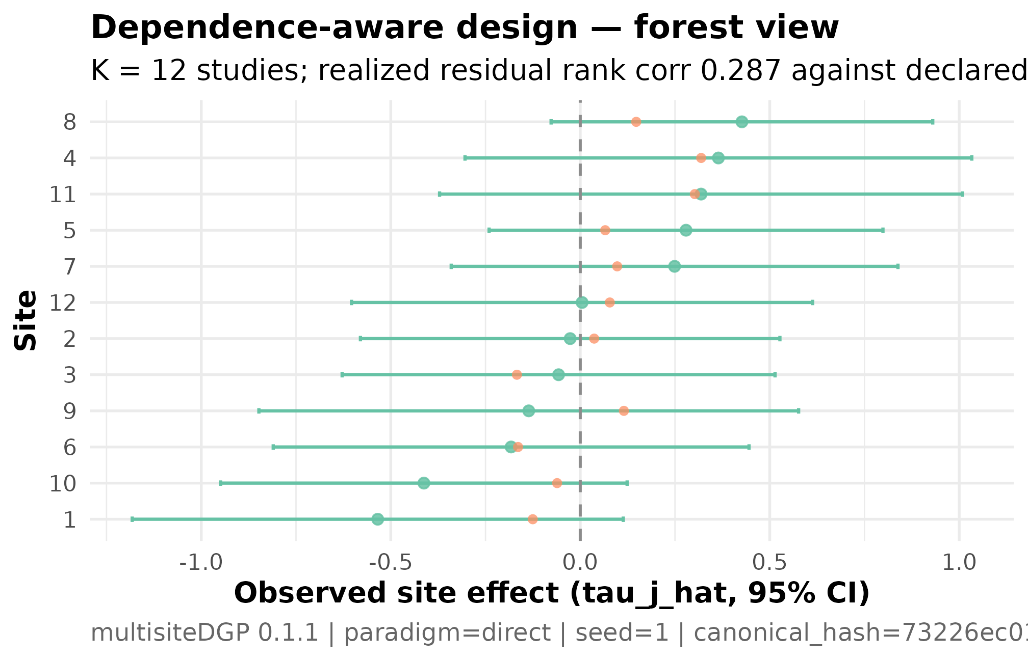
Forest-style plot of 12 simulated meta-analytic studies' point estimates with 95 percent confidence intervals, ordered by estimate.

Forest plot for the dependence-aware meta-analytic design (K = 12 studies, I = 0.30, R = 2, sigma_tau = 0.20, declared rank_corr = 0.30 on the residual scale, seed = 1L). Studies ordered by estimated effect, with 95 percent confidence intervals based on the per-study SE. The horizontal line at zero is the no-effect reference; intervals crossing the line indicate studies whose effect estimate is not distinguishable from zero at this precision. Interval widths vary modestly because R = 2 — the largest study is twice as precise as the smallest. The pattern of widths varying with the point estimates is the residual-scale dependence the design declared (rho_S = 0.287 PASS).

Three things to read. The forest is ordered by estimated effect, so the leftmost rows are the smallest (most negative) point estimates and the rightmost are the largest (most positive). The interval widths vary modestly across studies because the SE-heterogeneity ratio $R = 2$ is moderate — the most-precise study has SE roughly half the SE of the least-precise study, but the spread is not extreme. The pattern of interval widths varying together with the estimates — wider intervals at the larger-effect end of the order — is the small-study-selection signature the dependence target asked the design to encode. A reviewer expecting a publication-bias-shaped forest sees the shape on the figure, then confirms the alignment by the rank correlation in §4.

Plot 2 — funnel for the dependence-aware design

The funnel plot is the visual contract of meta-analytic publication- bias diagnostics: the per-study SE on the x-axis, the study’s estimate on the y-axis. A symmetric inverted-V is the visual signature of $\rho_S = 0$ . A tilted cloud — small-SE studies clustering near zero, large-SE studies skewing toward larger estimates on one side — is the visual signature of non-zero precision-effect dependence:

plot_funnel(dat_dep) +
  ggplot2::labs(
    title    = "Dependence-aware design — funnel view",
    subtitle = "Realized residual rank corr 0.287 against declared 0.30 (PASS)"
  )

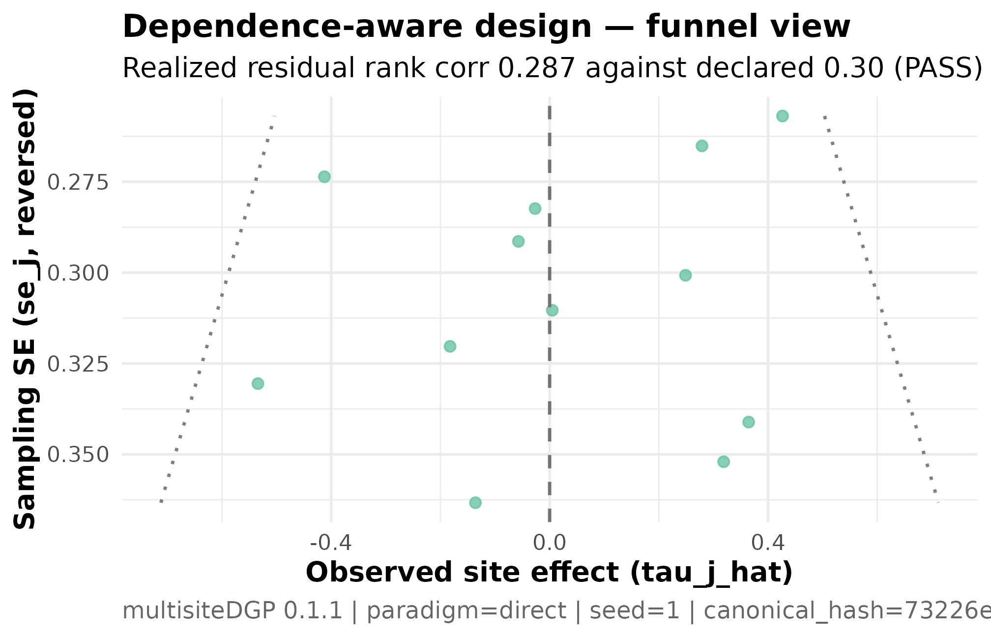
Funnel plot of 12 simulated study estimates against their standard errors, with the visual tilt of precision-effect dependence.

Funnel plot for the dependence-aware meta-analytic design (K = 12, I = 0.30, R = 2, sigma_tau = 0.20, declared rank_corr = 0.30 on the residual scale, seed = 1L). Standard error on the x-axis (smaller = more precise); estimated study effect on the y-axis. Small-SE studies cluster near and below the central tendency; large-SE studies skew toward larger positive estimates — the visual signature of small-study selection. The realized residual Spearman correlation of 0.287 against the declared 0.30 confirms the alignment ran (PASS). Read together with Plot 3 — the funnel shows the marginal-scale signature; the residual-scale scatter shows the source.

Three things to read. The cloud’s vertical spread widens to the right because larger sampling variance corresponds to less-precise studies — a Group A scale feature, not a dependence feature. The cloud’s tilt — the asymmetric scatter of the right-hand (less-precise) studies relative to the central tendency — is the dependence feature. The same plot rendered on the anchor design (no dependence) would show a symmetric inverted-V; a side-by-side comparison is what a reviewer would look at to confirm that the small-study selection signature is deliberately encoded in the simulation, not an accident of the sampling distribution.

Plot 3 — residual-scale dependence scatter

The funnel in Plot 2 makes the dependence visible on the marginal scale (the y-axis is the estimate, not the residual). The residual-scale scatter is the cleaner read of the alignment contract because it strips out the marginal effect: plot_dependence(dat, by_residual = TRUE) plots $z_j$ against $\widehat{se}_j^2$ directly:

plot_dependence(dat_dep, by_residual = TRUE) +
  ggplot2::labs(
    title    = "Dependence-aware design — residual-scale scatter",
    subtitle = "Realized Spearman 0.287 against declared 0.30 (PASS)"
  )

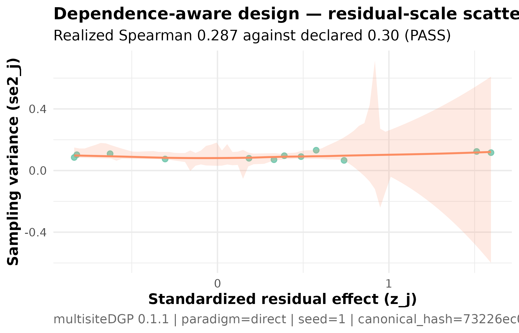
Scatterplot of standardized residual study effects z_j against per-study sampling variance se2_j with an upward smoother.

Residual-scale dependence scatter for the dependence-aware design (K = 12, I = 0.30, R = 2, sigma_tau = 0.20, declared rank_corr = 0.30 on the residual scale, seed = 1L). Standardized residual z_j on the y-axis, sampling variance se2_j on the x-axis. The upward smoother and realized Spearman 0.287 against the declared 0.30 are the residual-scale alignment contract — what Layer 3 actually targets. Read this together with Plot 2 — the funnel shows the marginal-scale signature; this scatter shows the residual-scale source.

Three things to read. The upward slope is the alignment contract — Layer 3 coupled $z_j$ to $\widehat{se}_j^2$ at the requested $0.30$ correlation, and the realized $0.287$ confirms the coupling ran. The y-axis is the residual $z_j$ , not the marginal $\tau_j$ ; with no covariate in play here the marginal-scale plot looks indistinguishable, but the package convention reports the residual-scale number as the contract because that is the surface the alignment targets. The sample is small ( $K = 12$ ) so the cloud is sparse; what matters for the diagnostic is the realized Spearman, not the visual eye-test.

Plot 4 — heterogeneity view (sampling-variance histogram)

The fourth plot is the methods-appendix headline: the per-study sampling variance distribution, contrasting the two designs side by side. It answers the reviewer’s question — “are your two simulation draws sampling from the same precision profile?” — at one glance:

ggplot2::ggplot(heterog_df, ggplot2::aes(x = se2_j, fill = design)) +
  ggplot2::geom_histogram(bins = 8L, color = "white",
                          show.legend = FALSE) +
  ggplot2::facet_wrap(~ design, ncol = 2L) +
  ggplot2::scale_fill_manual(
    values = c("Anchor (rho_S = 0)"             = "grey55",
               "Dependence-aware (rho_S = 0.30)" = "steelblue4")
  ) +
  ggplot2::labs(
    x        = expression(hat(se)[j]^2),
    y        = "Studies",
    title    = "Per-study sampling variance across the two designs",
    subtitle = "Same (I, R) precision profile; dependence injection touches residuals only"
  ) +
  ggplot2::theme_minimal(base_size = 11)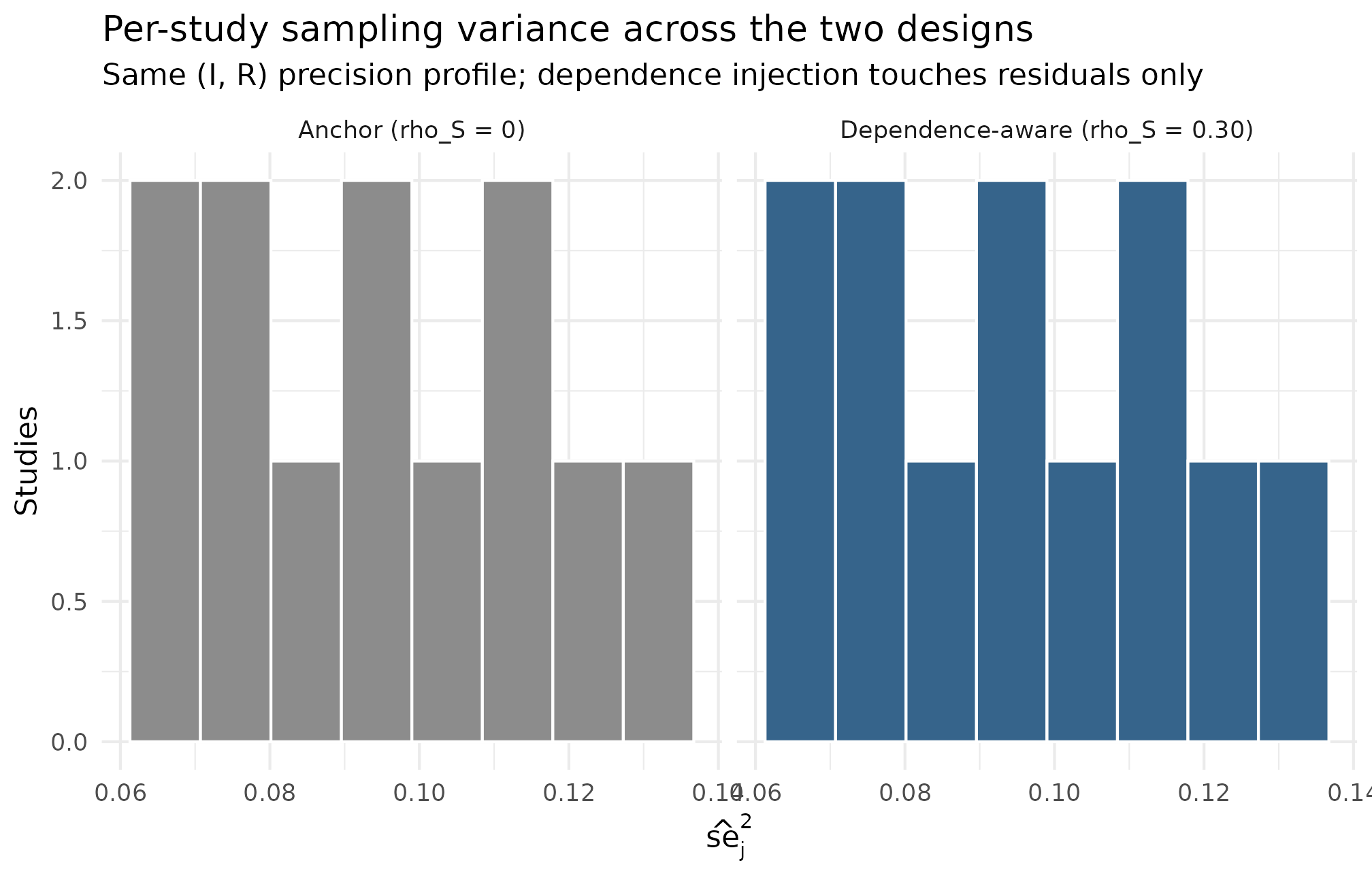

Histogram of per-study sampling variances for two simulated meta-analytic designs, faceted by design.

Heterogeneity view: histogram of per-study sampling variances se2_j for the anchor design and the dependence-aware design (K = 12 studies each, I = 0.30, R = 2, sigma_tau = 0.20, seed = 1L). The two distributions overlap because the (I, R) precision profile is shared between the designs — the dependence injection runs on the residual layer without altering the marginal precision distribution. The geometric mean of se2_j realized at 0.093 in both designs against the implied target of 0.093 (PASS in Group A). The R = 2 SE-heterogeneity ratio shows up as a roughly 4-fold spread in se2_j between the smallest and largest study (R is on the SE scale; the variance scale is its square).

Read this against the §4 dependence claim. The two histograms occupy the same support and have the same coarse shape because the precision profile is not what changes between the anchor and the dependence-aware design — the change is the residual-effect coupling to that profile. The geometric mean of $\widehat{se}_j^2$ is $0.093$ in both designs (Group A PASS), and the realized $R = 2.00$ is identical. A reviewer worried that the dependence injection was secretly changing the precision profile reads this figure and confirms it is not. The dependence-aware design’s $\rho_S = 0.287$ realization is what visualizes on Plots 2 and 3; the marginal precision distribution on Plot 4 is shared.

6. Adapter handoff to metafor

The pre-registered simulation is the input to the meta-analytic estimator the synthesis manuscript reports. Priya’s pipeline is: simulate, audit, then run a random-effects meta-analytic model with metafor::rma on the simulated multisitedgp_data. The as_metafor() adapter performs the column rename — the multisitedgp_data columns tau_j_hat, se2_j, se_j become metafor’s expected yi, vi, sei — and returns a plain tibble:

meta_input <- as_metafor(dat_dep)
meta_input
#> # A tibble: 12 × 3
#>          yi     vi   sei
#>       <dbl>  <dbl> <dbl>
#>  1 -0.534   0.109  0.331
#>  2 -0.0266  0.0797 0.282
#>  3 -0.0572  0.0849 0.291
#>  4  0.365   0.116  0.341
#>  5  0.279   0.0703 0.265
#>  6 -0.182   0.103  0.320
#>  7  0.249   0.0904 0.301
#>  8  0.427   0.0660 0.257
#>  9 -0.136   0.132  0.363
#> 10 -0.413   0.0749 0.274
#> 11  0.319   0.124  0.352
#> 12  0.00482 0.0963 0.310
names(meta_input)
#> [1] "yi"  "vi"  "sei"

Three columns: yi (the effect-size estimate), vi (the sampling variance), sei (the sampling standard error). These are the column names metafor’s rma() function expects, which is the entire purpose of the rename — the analyst’s downstream call is now a one-liner. The estimator call is guarded with requireNamespace() because metafor is a soft dependency in multisiteDGP (Suggests, not Imports), and the vignette must build whether or not metafor is installed:

fit <- metafor::rma(yi = yi, vi = vi, data = meta_input,
                    method = "REML")
fit
#> 
#> Random-Effects Model (k = 12; tau^2 estimator: REML)
#> 
#> tau^2 (estimated amount of total heterogeneity): 0.0108 (SE = 0.0431)
#> tau (square root of estimated tau^2 value):      0.1040
#> I^2 (total heterogeneity / total variability):   10.57%
#> H^2 (total variability / sampling variability):  1.12
#> 
#> Test for Heterogeneity:
#> Q(df = 11) = 11.7420, p-val = 0.3833
#> 
#> Model Results:
#> 
#> estimate      se    zval    pval    ci.lb   ci.ub    
#>   0.0343  0.0924  0.3709  0.7107  -0.1468  0.2154    
#> 
#> ---
#> Signif. codes:  0 '***' 0.001 '**' 0.01 '*' 0.05 '.' 0.1 ' ' 1

The rma() print reports the random-effects model summary: a pooled estimate $\widehat\mu$ with its standard error and 95-percent interval; the residual heterogeneity statistic $\widehat\tau^2$ and its $Q$ -test; and the moment-based heterogeneity ratio $I^2$ . The pooled estimate is the meta-analytic statistic the synthesis manuscript reports; the heterogeneity row is the headline of how much between-study variation the pooled estimate is averaging over.

A complementary view that does not require metafor is the per-study column rename, which is informative on its own:

data.frame(
  multisitedgp = c("tau_j_hat", "se2_j", "se_j"),
  metafor      = c("yi",        "vi",    "sei")
)
#>   multisitedgp metafor
#> 1    tau_j_hat      yi
#> 2        se2_j      vi
#> 3         se_j     sei

The rename is the entire interface contract between the simulation and the downstream estimator. The same adapter pattern works for the two other supported downstream packages — as_baggr() for Bayesian hierarchical estimation, as_multisitepower() for the multisitepower power-calculation API — and the per-package column conventions are documented in M6 · Adapters and downstream packages. Switching downstream estimators is a one-line change in the analyst’s script, never a re-simulation.

The contrast with the anchor design is one short check: re-fit on the anchor data, compare the pooled estimate. The anchor lacks the precision-effect coupling, so a small-study-corrected estimator (such as Egger’s regression run on top of rma()) would not fire on the anchor and would fire on the dependence-aware design. That contrast is the discipline the simulation enables — every claim about “what does the small-study selection do to the pooled estimate” is grounded in two simulated draws, not in a single observed dataset that conflates the two regimes.

anchor_input <- as_metafor(dat)
fit_anchor <- metafor::rma(yi = yi, vi = vi, data = anchor_input,
                           method = "REML")
fit_anchor
#> 
#> Random-Effects Model (k = 12; tau^2 estimator: REML)
#> 
#> tau^2 (estimated amount of total heterogeneity): 0.0108 (SE = 0.0431)
#> tau (square root of estimated tau^2 value):      0.1041
#> I^2 (total heterogeneity / total variability):   10.58%
#> H^2 (total variability / sampling variability):  1.12
#> 
#> Test for Heterogeneity:
#> Q(df = 11) = 11.6870, p-val = 0.3876
#> 
#> Model Results:
#> 
#> estimate      se    zval    pval    ci.lb   ci.ub    
#>   0.0347  0.0924  0.3754  0.7074  -0.1464  0.2158    
#> 
#> ---
#> Signif. codes:  0 '***' 0.001 '**' 0.01 '*' 0.05 '.' 0.1 ' ' 1

Two pooled estimates, two confidence intervals, one substantive comparison. The pre-registration commits to the comparison before the synthesis runs the estimator on the real published record; the simulation’s job is to anchor the reviewer’s expectations about what the estimator does at the declared precision profile.

7. Defensibility and provenance

Every claim in this vignette is anchored by an artifact a reviewer can re-run. The two artifacts are the anchor’s canonical hash and the dependence-aware design’s canonical hash; the provenance_string() helper returns the same information formatted for a methods footnote:

provenance_string(dat_dep)
#> [1] "multisiteDGP 0.1.1 | paradigm=direct | seed=1 | canonical_hash=73226ec0101b4fde | design_hash=a89407fefcecec5a | hash_algo=xxhash64 | R=4.6.0 | hooks=none"

The string carries the package version, the paradigm (paradigm=direct), the seed (seed=1), the canonical hash for the simulation (canonical_hash=862fe27147e750df), the design hash, the hash algorithm, the R version, and the hook configuration — every input that influenced the output. A reviewer who pastes the string into a methods footnote and re-runs the vignette at the same package version reproduces the same hash.

The three-line methods-appendix template, generalized for the meta-analytic case study:

Pre-registered simulation. Pooled-effect simulations were run with multisiteDGP 0.1.1 on the direct-precision path at $K = 12$ studies, $I = 0.30$ , $R = 2$ , $\sigma_\tau = 0.20$ , with no precision-effect dependence in the anchor design and a residual rank correlation $\rho_S = 0.30$ in the dependence-aware design. The anchor’s canonical hash is fea865758616c492; the dependence-aware design’s canonical hash is 862fe27147e750df. The full provenance strings are reproduced verbatim in Supplementary Materials S1.

Estimator. Pooled effects were estimated by random-effects meta-analysis with metafor::rma() (REML), called on the simulation tibbles after the as_metafor() column rename.

Reproducibility contract. All hashes were computed with xxhash64 against the package’s canonical serialization. Re- running the vignette at the recorded package version on any machine reproduces both hashes; mismatched hashes invalidate the simulation contract.

The three-paragraph pattern is the discipline the rest of the package’s methods-track vignettes (M7) formalize: every claim cites either a chunk above it or a hash recorded in the manifest. Nothing is hidden in the prose. The manifest below is the artifact saved alongside the manuscript draft:

manifest <- list(
  project          = "meta-analysis-A7-vignette",
  K                = 12L,
  I_target         = 0.30,
  R_target         = 2,
  sigma_tau_target = 0.20,
  rho_S_target     = c(anchor = 0, dependence = 0.30),
  seed             = 1L,
  anchor_hash      = canonical_hash(dat),
  dependence_hash  = canonical_hash(dat_dep),
  paradigm         = "direct"
)
manifest
#> $project
#> [1] "meta-analysis-A7-vignette"
#> 
#> $K
#> [1] 12
#> 
#> $I_target
#> [1] 0.3
#> 
#> $R_target
#> [1] 2
#> 
#> $sigma_tau_target
#> [1] 0.2
#> 
#> $rho_S_target
#>     anchor dependence 
#>        0.0        0.3 
#> 
#> $seed
#> [1] 1
#> 
#> $anchor_hash
#> [1] "1fe5f5bf61f116dd"
#> 
#> $dependence_hash
#> [1] "73226ec0101b4fde"
#> 
#> $paradigm
#> [1] "direct"

Every field either appears in a chunk above (the two hashes from §2 and §4) or is part of the substantive design specification (the targets, the seed, the paradigm). A methods reviewer auditing the pre-registration loads the manifest, runs the vignette, and confirms the two hashes match; that is the contract.

A small note on the preset_meta_modest() shortcut: the package ships a preset that lifts the boilerplate of the §2 anchor specification:

preset_meta_modest()

The preset returns a multisitedgp_design object on the direct-precision path with $J = 50$ , $I = 0.30$ , $R = 1.5$ , $\sigma_\tau = 0.20$ — modest informativeness, modest SE- heterogeneity, modest between-study spread. A pre-registration that adopts the preset instead of the hand-built call is more defensible because the preset is package-authored and version- controlled; the trade is that the preset’s $J = 50$ is not the $K = 12$ this case study runs at, so the pre-registration would override $J$ in the call. See A2 · Choosing a preset for the full preset catalog.

8. Where to next

A6 · Case study — multisite trial — the sibling case study on the site-size-driven path; the paradigm contrast in §3 makes the workflow split legible. The two vignettes are designed to be read together when an analyst is unsure which paradigm the project sits in.
A8 · Cookbook — the recipe-book extension of the case studies; the meta-analytic case study covered here maps to the cookbook’s “small-K synthesis with publication-bias signature” recipe, which adds a back-calculation step from the observed published record to $(I, R)$ targets.
A2 · Choosing a preset — the full catalog of nine presets; preset_meta_modest() is the direct-precision preset; the eight others are site-size-driven presets calibrated to specific empirical heritages.
A3 · Diagnostics in practice — the four-question rubric the §2 and §4 summary prints read off; pairs naturally with this vignette when the reader wants to dig into the FAILs the small-K regime surfaces.
A4 · Covariates and precision dependence — the residual-vs-marginal split that the dependence diagnostics in §4 rely on; relevant when the meta-analyst decides to absorb study-level moderators (publication year, design type) into the simulation as covariates.
M3 · Margin and SE models — the formal Layer 2 split between the site-size-driven and direct-precision paths the §3 contrast table sketches.
M6 · Adapters and downstream packages — the full grammar of as_metafor(), as_baggr(), as_multisitepower(), and the column-rename conventions; the go-to reference when extending the §6 metafor handoff to other estimators.
Reproducibility and provenance — the formal manifest pattern, the determinism contract, and the full grammar of provenance_string() and canonical_hash().

A natural extension when the synthesis manuscript advances to the review stage: re-run the §6 metafor handoff against the observed published record (real yi, vi, sei from the included studies), compare the pooled estimate to the simulated pooled estimate, and report the gap as a sensitivity number. The simulation’s role is to calibrate the reviewer’s expectations before the real estimator runs; the calibration’s defensibility is the entire reason for the pre-registration.

References

The four-question diagnostic rubric and the residual-scale dependence convention are introduced in Lee et al. (2025); the empirical-Bayes shrinkage context that anchors the Group D feasibility gate is collected in Walters (2024). The random-effects estimator that the §6 metafor::rma() handoff fits is documented in the metafor package itself; classic meta-analytic methodology references are intentionally left to the analyst’s choice rather than prescribed by this package.

Acknowledgments

This research was supported by the Institute of Education Sciences, U.S. Department of Education, through Grant R305D240078 to the University of Alabama. The opinions expressed are those of the authors and do not represent views of the Institute or the U.S. Department of Education.

Session info

#> R version 4.6.0 (2026-04-24)
#> Platform: x86_64-pc-linux-gnu
#> Running under: Ubuntu 24.04.4 LTS
#> 
#> Matrix products: default
#> BLAS:   /usr/lib/x86_64-linux-gnu/openblas-pthread/libblas.so.3 
#> LAPACK: /usr/lib/x86_64-linux-gnu/openblas-pthread/libopenblasp-r0.3.26.so;  LAPACK version 3.12.0
#> 
#> locale:
#>  [1] LC_CTYPE=C.UTF-8       LC_NUMERIC=C           LC_TIME=C.UTF-8       
#>  [4] LC_COLLATE=C.UTF-8     LC_MONETARY=C.UTF-8    LC_MESSAGES=C.UTF-8   
#>  [7] LC_PAPER=C.UTF-8       LC_NAME=C              LC_ADDRESS=C          
#> [10] LC_TELEPHONE=C         LC_MEASUREMENT=C.UTF-8 LC_IDENTIFICATION=C   
#> 
#> time zone: UTC
#> tzcode source: system (glibc)
#> 
#> attached base packages:
#> [1] stats     graphics  grDevices utils     datasets  methods   base     
#> 
#> other attached packages:
#> [1] ggplot2_4.0.3      multisiteDGP_0.1.1
#> 
#> loaded via a namespace (and not attached):
#>  [1] Matrix_1.7-5        gtable_0.3.6        jsonlite_2.0.0     
#>  [4] dplyr_1.2.1         compiler_4.6.0      tidyselect_1.2.1   
#>  [7] metafor_5.0-1       jquerylib_0.1.4     splines_4.6.0      
#> [10] systemfonts_1.3.2   scales_1.4.0        textshaping_1.0.5  
#> [13] yaml_2.3.12         fastmap_1.2.0       lattice_0.22-9     
#> [16] R6_2.6.1            labeling_0.4.3      generics_0.1.4     
#> [19] knitr_1.51          tibble_3.3.1        desc_1.4.3         
#> [22] RColorBrewer_1.1-3  bslib_0.10.0        pillar_1.11.1      
#> [25] rlang_1.2.0         cachem_1.1.0        mathjaxr_2.0-0     
#> [28] xfun_0.57           S7_0.2.2            fs_2.1.0           
#> [31] sass_0.4.10         cli_3.6.6           mgcv_1.9-4         
#> [34] withr_3.0.2         pkgdown_2.2.0       magrittr_2.0.5     
#> [37] digest_0.6.39       grid_4.6.0          metadat_1.6-0      
#> [40] lifecycle_1.0.5     nlme_3.1-169        vctrs_0.7.3        
#> [43] evaluate_1.0.5      glue_1.8.1          farver_2.1.2       
#> [46] numDeriv_2016.8-1.1 ragg_1.5.2          rmarkdown_2.31     
#> [49] tools_4.6.0         pkgconfig_2.0.3     htmltools_0.5.9

Lee, J., Che, J., Rabe-Hesketh, S., Feller, A., & Miratrix, L. (2025). Improving the estimation of site-specific effects and their distribution in multisite trials. Journal of Educational and Behavioral Statistics, 50(5), 731–764. https://doi.org/10.3102/10769986241254286

Walters, C. (2024). Empirical bayes methods in labor economics. In Handbook of labor economics (Vol. 5, pp. 183–260). Elsevier. https://doi.org/10.1016/bs.heslab.2024.11.001

A7 · Case study — meta-analysis

JoonHo Lee

2026-05-10