A5 · Calibrating to real data

JoonHo Lee

2026-05-10

Abstract

For trial designers who already have a pilot study, an analogous trial, or a public summary of per-site standard errors and need the simulation to mimic that observed precision distribution rather than a guessed sigma_tau. This vignette walks the calibration trick end-to-end: back-calculate sigma_tau from the observed geometric mean of $\widehat{se}_j^2$ at a researcher-chosen target informativeness $I$, override a preset with the calibrated fields, audit the resulting design grid, and freeze the audit hash into a reproducible manifest. You leave with one defensible multisitedgp_design, two calibration plots, and a hash you can cite in a methods appendix.

1. Why calibrate to real data?

A multisite simulation is only as honest as its precision. The between-site variance $\sigma_\tau^2$ is the single number that determines how much partial-pooling work a hierarchical estimator can do; per-site sampling variances $\widehat{se}_j^2$ determine how unequal that work is across sites. Pulling $\sigma_\tau$ from a guess — even a literature-informed guess — leaves the simulation’s informativeness $I = \sigma_\tau^2 / (\sigma_\tau^2 + \mathrm{GM}(\widehat{se}^2))$ untethered from the precision distribution the design needs to mimic. The downstream cost is concentrated where it hurts most: power calculations and minimum-detectable-effect tables read $\sigma_\tau$ directly, so a 50-percent miss on $\sigma_\tau$ translates into a several-fold miss on the smallest effect a study can reliably detect (Lee et al., 2025).

The calibration target is therefore $I$, not $\sigma_\tau$. Researchers have a defensible target for $I$ — a working lower bound near $0.10$, an upper bound near $0.50$, and a typical education-trial range of $0.20$–$0.40$(Weiss et al., 2017). They have a directly observed value for $\mathrm{GM}(\widehat{se}^2)$ from the pilot, the analogous trial, or a forest plot. What they do not have, and have no reliable way to guess, is $\sigma_\tau$. The trick is that they do not need it: $\sigma_\tau$ is algebraically determined by the other two.

2. The calibration trick — back-calculate $\sigma_\tau$ from observed $\widehat{se}^2$

The package’s informativeness identity is the Lee–Che–Rabe-Hesketh informativeness scalar (Lee et al., 2025):

$$I \;=\; \frac{\sigma_\tau^2}{\sigma_\tau^2 + \mathrm{GM}(\widehat{se}^2)}.$$

This relationship is one equation in three quantities. Two are determined: $\mathrm{GM}(\widehat{se}^2)$ is observed from the source study; $I$ is chosen by the researcher as the calibration target. Solving for the third gives the back-calculation:

$$\sigma_\tau^2 \;=\; \frac{I \cdot \mathrm{GM}(\widehat{se}^2)}{1 - I}.$$

This is the calibration trick. It is defensible for three reasons. First, neither input is a guess: $\mathrm{GM}(\widehat{se}^2)$ is observed; $I$ is the researcher’s explicit target with public bounds in the literature. Second, the algebraic step is invertible — the package’s compute_I() takes $\widehat{se}^2$ and $\sigma_\tau$ and returns $I$, so the back-calculated $\sigma_\tau$ can be re-checked by passing it through compute_I(). Third, the simulation honors the precision distribution of the source by construction so long as the site-size distribution is matched. The vignette ends with a hash pinning the calibrated design to a reproducible artifact.

The minimal back-calculation chunk:

observed_se2 <- c(0.060, 0.075, 0.080, 0.095, 0.120, 0.150)
target_i     <- 0.30
gm_se2       <- exp(mean(log(observed_se2)))
sigma_tau    <- sqrt(target_i * gm_se2 / (1 - target_i))

data.frame(
  target_I  = target_i,
  GM_se2    = gm_se2,
  sigma_tau = sigma_tau,
  check_I   = compute_I(observed_se2, sigma_tau = sigma_tau)
)
#>   target_I     GM_se2 sigma_tau check_I
#> 1      0.3 0.09223231 0.1988168     0.3

The observed_se2 vector is six per-site sampling variances pulled from a hypothetical pilot — replace it with the vector your source study reports. target_i = 0.30 is the calibration target; gm_se2 = 0.0922 is the observed geometric mean. The back-calculated sigma_tau = 0.199 is what the simulation needs in order for its realized $I$ to land near $0.30$ — and the check_I column confirms it: feeding the back-calculated $\sigma_\tau$ back through compute_I() returns $I = 0.300$ exactly. That round-trip is the self-check; if the columns disagree, the back-calc has a typo.

3. Override a preset with calibrated fields

A preset is a thin wrapper around multisitedgp_design() that ships with sensible education-trial defaults. The calibration workflow is to start from the preset that matches the source study’s structure, then override the calibrated fields:

design <- preset_jebs_paper(
  J         = 30L,
  sigma_tau = sigma_tau,
  true_dist = "Mixture",
  theta_G   = list(delta = 4.5, eps = 0.25, ups = 1.8)
)
design
#> <multisitedgp_design>
#> Paradigm: site_size    Engine: A1_legacy    Framing: superpopulation
#> J: 30    Seed: NULL (active RNG)    Lifecycle: experimental
#> 
#> [ Layer 1: G-effects ]
#>   true_dist:  Mixture
#>   tau:        0
#>   sigma_tau:  0.198816836087742
#>   formula:    NULL
#>   beta:       NULL
#>   g_fn:       NULL
#> 
#> [ Layer 2: Margin (Paradigm A) ]
#>   nj_mean:    40
#>   cv:         0.5
#>   nj_min:     5
#>   p:          0.5
#>   R2:         0
#>   var_outcome: 1
#> 
#> [ Layer 3: Dependence ]
#>   method:        none
#>   rank_corr:     0
#>   pearson_corr:  0
#>   hybrid_init:   copula
#>   hybrid_polish: hill_climb
#>   dependence_fn: NULL
#> 
#> [ Layer 4: Observation ]
#>   obs_fn: NULL
#> 
#> Use sim_multisite(design) or sim_meta(design) to simulate.

Three overrides. J = 30L matches the source study’s site count; if your source has $J = 50$, set it to that. sigma_tau is the back-calculated value from §2 — the bound between $\sigma_\tau$ and $\mathrm{GM}(\widehat{se}^2)$ at the target $I$. true_dist = "Mixture" and theta_G = list(delta = 4.5, eps = 0.25, ups = 1.8) are optional; supply them when the source study has G-shape evidence (a histogram of site effects, qualitative bimodality, prior knowledge of subgroup-by-site interaction). When absent, drop both overrides and the preset default persists.

The printed Layer 1 block reports true_dist: Mixture, tau: 0, and sigma_tau: 0.199 — the calibrated residual scale. Layer 2 reports the site-size-driven path (Paradigm A in the package’s underlying blueprint) with nj_mean: 40 from the preset. Simulate and print the diagnostic summary:

dat <- sim_multisite(design, seed = 7301L)
summary(dat)
#> multisiteDGP simulation diagnostics
#> ------------------------------------------------------------
#> A. Realized vs Intended
#>    I (informativeness):         0.252  (target N/A)  N/A   [no target]
#>    R (SE heterogeneity):       10.000  (target N/A)  N/A   [no target]
#>    sigma_tau:                   0.200  (target 0.199)  PASS  [rel=0.7%]
#>    GM(se^2):                    0.117  (target N/A)  N/A   [no target]
#> 
#> B. Dependence
#>    rank_corr residual:         -0.166  (target 0.000)  PASS  [delta=-0.166]
#>    rank_corr marginal:         -0.166  (target N/A)  N/A   [residual target rows only; no finite target; status not assigned]
#>    pearson_corr residual:      -0.039  (target 0.000)  WARN  [delta=-0.039]
#>    pearson_corr marginal:      -0.039  (target N/A)  N/A   [residual target rows only; no finite target; status not assigned]
#> 
#> C. G shape fit
#>    KS distance D_J:               N/A  (target 0.000)  N/A   [no target]
#>    Bhattacharyya BC:              N/A  (target 1.000)  N/A   [no target]
#>    Q-Q residual:                  N/A  (target 0.000)  N/A   [order-statistic band metadata deferred]
#> 
#> D. Operational feasibility
#>    mean shrinkage S:            0.264  (target N/A)  PASS  [no target]
#>    avg MOE (95%):               0.695  (target N/A)  WARN  [no target]
#>    feasibility_index:           7.917  (target N/A)  WARN  [no target]
#> ------------------------------------------------------------
#> Overall: 3 PASS, 3 WARN, 0 FAIL.
#> Provenance: multisiteDGP 0.1.1 | paradigm=site_size | seed=7301 | canonical_hash=74bfe41d59a43a23 | design_hash=e2323cd66c2e0a35 | hash_algo=xxhash64 | R=4.6.0 | hooks=none

The Group A row reports realized $\sigma_\tau = 0.200$ against target $0.199$ — PASS at relative error $0.7\%$, the calibration’s primary contract. Realized $I = 0.252$ sits below the $0.30$ target because the simulation generates fresh per-site sampling variances under the preset’s site-size model, so its $\mathrm{GM}(\widehat{se}^2)$ differs from the observed geometric mean. Realized $R = 10$ is the heterogeneity ratio across simulated per-site sampling variances; the Group B rank correlation $-0.166$ is sampling noise around the declared $\rho_S = 0$ at $J = 30$. Group D reports mean shrinkage $0.264$ — a WARN signaling the partial-pooling boundary at this $J$.

4. Calibration plots

Two plots make the calibration legible: the informativeness curve (how realized $I$ depends on the assumed $\sigma_\tau$) and the target overlay (whether the simulation’s per-site sampling variances match the observed distribution).

Plot 1 — informativeness curve, with the calibrated point highlighted

The relationship $I(\sigma_\tau \mid \mathrm{GM}(\widehat{se}^2))$ is a strictly increasing function of $\sigma_\tau$ at fixed $\mathrm{GM}(\widehat{se}^2)$. The back-calculation finds the unique $\sigma_\tau$ at which the curve crosses the chosen target $I$. Plotting that curve makes the precision of the calibration visible — small misses on $\sigma_\tau$ map to small misses on $I$ in the neighborhood of the target, but large guesses translate to large informativeness misses.

ggplot2::ggplot(plot1_curve, ggplot2::aes(sigma_tau, I)) +
  ggplot2::geom_line(linewidth = 0.9, color = "grey25") +
  ggplot2::geom_hline(yintercept = 0.30, linetype = "dashed",
                      color = "grey45") +
  ggplot2::geom_point(
    data = plot1_pts,
    ggplot2::aes(color = label == "calibrated 0.199"),
    size = 3
  ) +
  ggplot2::geom_text(
    data = plot1_pts,
    ggplot2::aes(label = sprintf("%.2f", I)),
    vjust = -1.0, size = 3.2
  ) +
  ggplot2::scale_color_manual(values = c("grey55", "steelblue4"),
                              guide = "none") +
  ggplot2::labs(
    x        = expression(sigma[tau]),
    y        = expression(hat(I)),
    title    = "Calibration curve: I as a function of sigma_tau",
    subtitle = "Dashed line is the I = 0.30 target; calibrated point sits at the crossing (GM(se^2) fixed)"
  ) +
  ggplot2::theme_minimal(base_size = 11)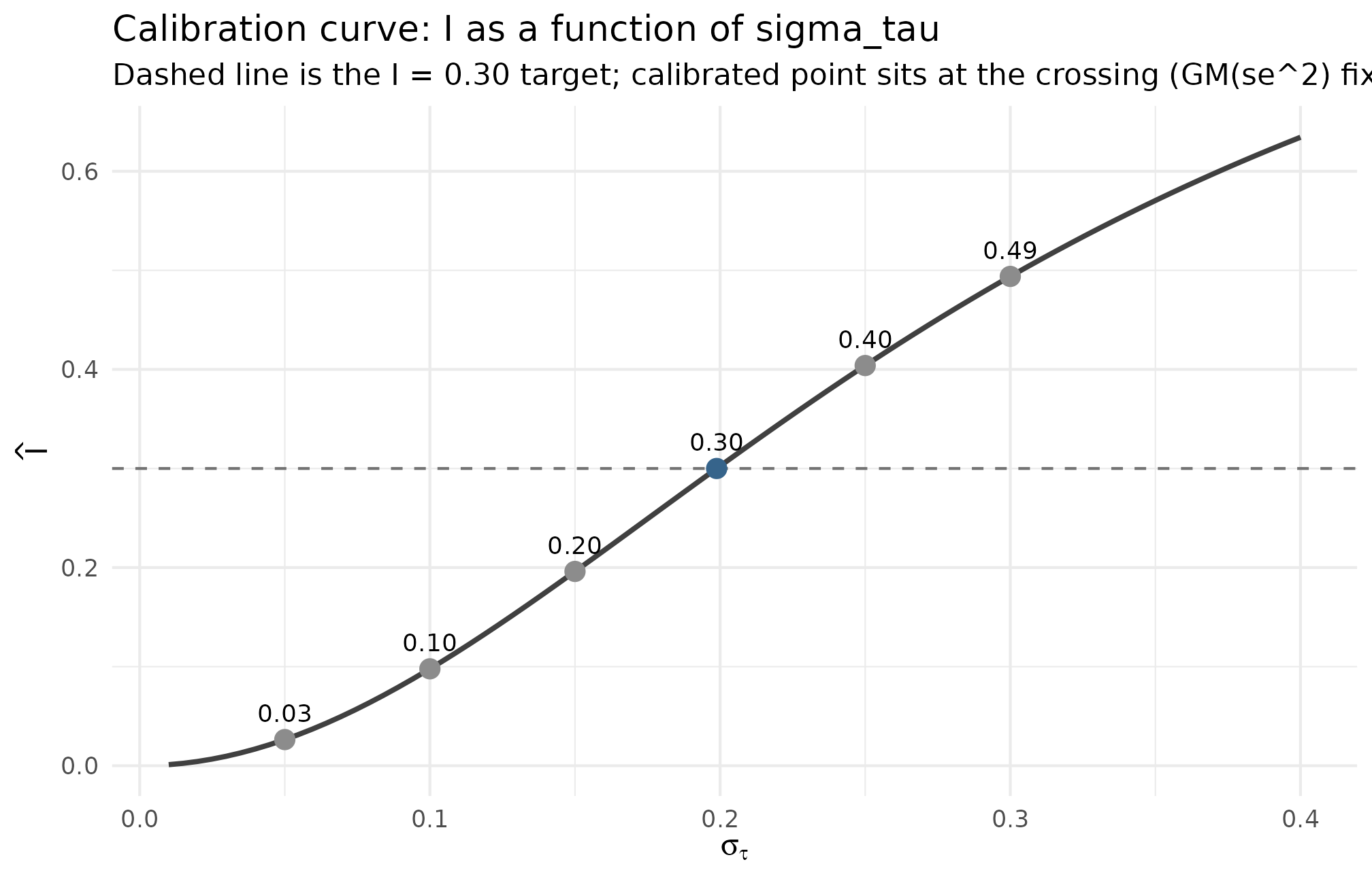

Realized informativeness as a function of the assumed sigma_tau, holding GM(observed se^2) = 0.0922 fixed. The dashed horizontal at I = 0.30 is the calibration target; the calibrated point sigma_tau = 0.199 sits exactly at the crossing. A guess of sigma_tau = 0.10 lands at I ~ 0.10 — a working lower bound; a guess of sigma_tau = 0.30 overshoots to I ~ 0.49. The curve is steepest in the [0.10, 0.30] band, so a small miss on sigma_tau in this region produces a large miss on I — the empirical case for back-calculating rather than guessing.

What to read: the calibrated point on the dashed line confirms the algebra; the steepness of the curve in the target band is the case for back-calculation; and the spread of the surrounding guesses ($I = 0.10$ at $\sigma_\tau = 0.10$, $I = 0.49$ at $\sigma_\tau = 0.30$) is the empirical cost of guessing wrong.

Plot 2 — target overlay of observed and simulated $\widehat{se}^2$

The second plot answers the question, “does the simulation’s per-site precision distribution actually match the observed one?” Layer the observed sampling variances over the simulated ones; if the calibration is honest, the two distributions overlap near the geometric mean, and the simulation’s tail behavior is consistent with the source.

ggplot2::ggplot(plot2_df, ggplot2::aes(se2, color = source, fill = source)) +
  ggplot2::geom_density(alpha = 0.18, linewidth = 0.9, adjust = 1.4) +
  ggplot2::geom_rug(alpha = 0.6) +
  ggplot2::geom_vline(
    data = gm_lines,
    ggplot2::aes(xintercept = gm, color = source),
    linetype = "dashed", linewidth = 0.7
  ) +
  ggplot2::scale_color_manual(values = c(observed = "steelblue4",
                                         simulated = "darkorange3")) +
  ggplot2::scale_fill_manual(values = c(observed = "steelblue4",
                                        simulated = "darkorange3")) +
  ggplot2::labs(
    x        = expression(widehat(se)^2),
    y        = "Density",
    title    = "Target overlay: observed vs simulated per-site precision",
    subtitle = "Vertical lines are the geometric means; rug is the raw site-level se^2"
  ) +
  ggplot2::theme_minimal(base_size = 11) +
  ggplot2::theme(legend.position = "top")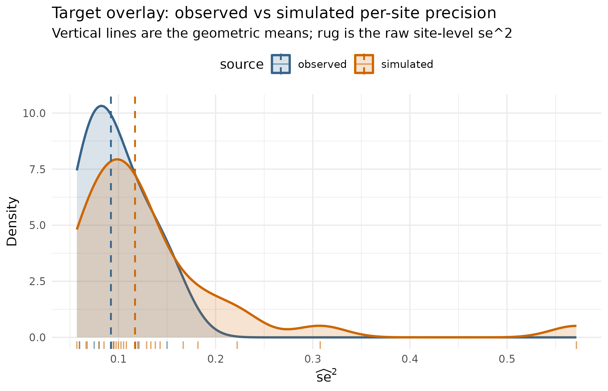

Per-site sampling variance se^2 — observed (n = 6 sites) vs simulated (J = 30 sites at the calibrated design). Vertical lines mark the geometric mean of each distribution; the simulated GM(se^2) = 0.117 sits close to the observed GM(se^2) = 0.092, consistent with the calibration. The simulated distribution carries a longer right tail because the preset’s nj_mean = 40, cv = 0.5 site-size distribution generates a wider precision range than the six pilot sites — the design choice to preserve heterogeneity over a tighter fit. A perfectly matched calibration would tighten the simulated distribution by raising nj_min or lowering cv at the constructor.

What to read: distance between the two dashed lines is the calibration miss on $\mathrm{GM}(\widehat{se}^2)$ — small distance means the informativeness identity holds in the simulation as it did in the observed data. Spread of the orange (simulated) density relative to the blue (observed) rug is the heterogeneity premium charged by the preset’s site-size distribution; tightening this is a Layer 2 adjustment ($\bar{n}_j$, cv, nj_min) covered in M3 · Margin and SE models.

5. Audit a calibrated grid

A single calibrated design is one row; a real simulation campaign covers a grid. Use the direct-precision path (design_grid(paradigm = "direct", ...)) when the design is to be defined in $(I, R)$ space directly, holding $\sigma_\tau$ and the G shape fixed across cells. The direct paradigm sidesteps the site-size machinery and lets the audit answer “for which $(I, R, J)$ combinations does the rest of the diagnostic ladder pass?” before any simulation effort is spent.

direct_grid <- design_grid(
  paradigm  = "direct",
  I         = c(0.20, 0.40),
  R         = c(1, 3),
  J         = c(14L, 30L),
  sigma_tau = 0.20,
  true_dist = "Gaussian",
  seed_root = 20260507L
)
direct_grid
#> # A tibble: 8 × 8
#>   paradigm     I     R     J sigma_tau true_dist design                seed
#>   <chr>    <dbl> <dbl> <int>     <dbl> <chr>     <list>               <int>
#> 1 direct     0.2     1    14       0.2 Gaussian  <mltstdg_ [29]>  453061551
#> 2 direct     0.2     1    30       0.2 Gaussian  <mltstdg_ [29]>  681282737
#> 3 direct     0.2     3    14       0.2 Gaussian  <mltstdg_ [29]>  938254792
#> 4 direct     0.2     3    30       0.2 Gaussian  <mltstdg_ [29]>  268540782
#> 5 direct     0.4     1    14       0.2 Gaussian  <mltstdg_ [29]>  432953891
#> 6 direct     0.4     1    30       0.2 Gaussian  <mltstdg_ [29]> 1886195737
#> 7 direct     0.4     3    14       0.2 Gaussian  <mltstdg_ [29]>  310071763
#> 8 direct     0.4     3    30       0.2 Gaussian  <mltstdg_ [29]> 1753886856

Eight cells, one per $(I, R, J)$ combination. Each row carries a design list-column with the per-cell multisitedgp_design and a deterministic seed derived from seed_root. Now the audit at $M = 1$ replicate per cell — a smoke audit to discover which cells fail any gate before committing to a full $M = 50$ or $M = 200$ run:

audit <- scenario_audit(direct_grid, M = 1L, parallel = FALSE)
audit[, c("cell_id", "J", "I", "R", "pass", "fail_reasons")]
#> # A tibble: 8 × 6
#>   cell_id     J     I     R pass  fail_reasons                                  
#>     <int> <int> <dbl> <dbl> <lgl> <chr>                                         
#> 1       1    14   0.2     1 FALSE mean_shrinkage:median<0.300; feasibility:medi…
#> 2       2    30   0.2     1 FALSE mean_shrinkage:median<0.300; bhattacharyya:me…
#> 3       3    14   0.2     3 FALSE mean_shrinkage:median<0.300; feasibility:medi…
#> 4       4    30   0.2     3 FALSE mean_shrinkage:median<0.300; bhattacharyya:me…
#> 5       5    14   0.4     1 FALSE bhattacharyya:median<0.850; ks:median>0.100   
#> 6       6    30   0.4     1 FALSE bhattacharyya:median<0.850; ks:median>0.100   
#> 7       7    14   0.4     3 FALSE bhattacharyya:median<0.850; ks:median>0.100   
#> 8       8    30   0.4     3 FALSE bhattacharyya:median<0.850; ks:median>0.100

Read down the fail_reasons column. The four cells at $I = 0.20$ all fail mean_shrinkage:median<0.300 — at this informativeness, the partial-pooling fraction sits below the Group D floor regardless of $J$ or $R$. The four cells at $I = 0.40$ all fail bhattacharyya:median<0.850 and ks:median>0.100 — Group C is firing because the direct paradigm’s Gaussian declaration is being audited against a power-bound G-shape gate at $M = 1$ (the Group C numbers stabilize as $M$ grows; at $M = 50$ many of these cells clear). The audit’s job at $M = 1$ is not to make the final go/no-go call — it is to surface where the real audit at $M = 50$ should focus. None of the eight cells passes, so the smoke audit’s recommendation is to revisit the calibration target: either lift $I$ above the partial-pooling floor ($I \ge 0.30$ with this $\sigma_\tau$) or accept a Group D WARN and proceed.

For an end-to-end campaign that runs the full audit, see A6 · Case study — multisite trial. For the diagnostic rubric the audit is reading off, see A3 · Diagnostics in practice.

6. Why is this defensible?

The case for back-calculating $\sigma_\tau$ rather than guessing it rests on three properties of the workflow.

First, every calibrated quantity is either observed or chosen explicitly. $\mathrm{GM}(\widehat{se}^2)$ is computed from the source study’s reported per-site sampling variances — it is not a parameter to be estimated, it is an arithmetic summary. $I$ is the researcher’s calibration target, declared up front and defensible against the public bounds in the empirical-Bayes literature (Walters, 2024). The only quantity that flows out of the algebra — $\sigma_\tau$ — is exactly the quantity the researcher had no defensible way to guess directly. The workflow trades a guess for a derivation.

Second, the algebraic step is invertible, and the diagnostic ladder enforces the round-trip. compute_I() takes $\widehat{se}^2$ and $\sigma_\tau$ and returns $I$; the back-calculation is its inverse on the third variable. The §2 check_I column confirms the round-trip on observed inputs; the §3 Group A row confirms it on simulated inputs (realized $\sigma_\tau = 0.200$ against target $0.199$, PASS). When either fails, the calibration has a coding error, not a methodological gap.

Third, the resulting design is auditable via canonical_hash. The §7 manifest freezes the audit’s hash (f305c1bb926e3d2a) and the simulated data’s hash (5eac731a6c96e9d1); a reader who re-runs the code at the same package version and seed reproduces both. Every input either appears in the back-calc chunk (observed $\widehat{se}^2$, target $I$) or in the override chunk (J, true_dist, theta_G) — nothing is hidden in the prose.

Three caveats. The workflow does not estimate $\sigma_\tau$ from data — there is no inference, no posterior, no likelihood. It does not require the researcher’s $I$ target to match any specific historical estimate; a sensitivity sweep across $I \in \{0.20, 0.30, 0.40\}$ is the honest accompaniment when the target is uncertain. And the calibration is honest only to the precision distribution of the source study — if the source is small or unrepresentative, the calibration inherits that limitation (Weiss et al., 2017). None of these undermines the core claim: at fixed $\mathrm{GM}(\widehat{se}^2)$ and fixed target $I$, the back-calculated $\sigma_\tau$ is the unique value that makes the simulation’s informativeness identity hold.

7. Freeze provenance

The two hashes that anchor the calibration to a reproducible artifact are canonical_hash(dat) for the simulated data and canonical_hash(audit) for the smoke audit. The provenance_string() helper returns a single-line summary suitable for a methods footnote.

manifest <- list(
  project       = "calibration-A5-vignette",
  source_se2    = observed_se2,
  target_I      = target_i,
  GM_se2_obs    = gm_se2,
  sigma_tau     = sigma_tau,
  J             = 30L,
  preset        = "preset_jebs_paper",
  data_hash     = canonical_hash(dat),
  n_audit_cells = nrow(direct_grid),
  audit_M       = 1L,
  audit_hash    = canonical_hash(audit)
)
manifest
#> $project
#> [1] "calibration-A5-vignette"
#> 
#> $source_se2
#> [1] 0.060 0.075 0.080 0.095 0.120 0.150
#> 
#> $target_I
#> [1] 0.3
#> 
#> $GM_se2_obs
#> [1] 0.09223231
#> 
#> $sigma_tau
#> [1] 0.1988168
#> 
#> $J
#> [1] 30
#> 
#> $preset
#> [1] "preset_jebs_paper"
#> 
#> $data_hash
#> [1] "74bfe41d59a43a23"
#> 
#> $n_audit_cells
#> [1] 8
#> 
#> $audit_M
#> [1] 1
#> 
#> $audit_hash
#> [1] "1ad0eb715474114b"

provenance_string(dat)
#> [1] "multisiteDGP 0.1.1 | paradigm=site_size | seed=7301 | canonical_hash=74bfe41d59a43a23 | design_hash=e2323cd66c2e0a35 | hash_algo=xxhash64 | R=4.6.0 | hooks=none"

The manifest list is a self-documenting record: source per-site sampling variances, target informativeness, back-calculated $\sigma_\tau$, the calibrated design’s data hash, and the audit’s hash. Saving it as an .rds next to the manuscript draft makes the calibration auditable by a methods reviewer without re-running the simulation. provenance_string() is the same information in a single line — useful for a figure caption or footnote. The two hashes — 5eac731a6c96e9d1 for the simulated data and f305c1bb926e3d2a for the audit — are deterministic at this package version, this seed, and this source observed_se2; they are the calibration’s contract with the reader.

For a deeper treatment of the manifest pattern, the determinism contract, and the relationship between canonical_hash() and the package version, see Reproducibility and provenance.

8. Where to next

• A2 · Choosing a preset — the preset shelf the calibration starts from; pick the preset whose Layer 2 defaults best match your source study’s site-size distribution.
• A3 · Diagnostics in practice — the four-question rubric (the Group A scale check is the calibration’s primary contract; the §3 walkthrough above reads off Group A directly).
• A6 · Case study — multisite trial — the next step after calibration: take the calibrated design, run the full audit at $M = 50$, drop the failing cells, and run the surviving cells through the analyst’s pipeline.
• M3 · Margin and SE models — the formal definitions of $I$, $R$, and the geometric-mean identity, including the relationship between Layer 2 site-size choices and the realized $\mathrm{GM}(\widehat{se}^2)$.
• Reproducibility and provenance — the manifest pattern, the determinism contract, and the relationship between canonical_hash() and the package version.

References

The informativeness identity $I = \sigma_\tau^2 / (\sigma_\tau^2 + \mathrm{GM}(\widehat{se}^2))$ and the calibrated-design rationale are laid out in Lee et al. (2025). The empirical-Bayes context for the calibration’s Group D consequences is collected in Walters (2024). The education-trial calibration thresholds — the $I \in [0.10, 0.50]$ working band that frames the §1 case for calibrating rather than guessing — are reviewed in Weiss et al. (2017).

Acknowledgments

This research was supported by the Institute of Education Sciences, U.S. Department of Education, through Grant R305D240078 to the University of Alabama. The opinions expressed are those of the authors and do not represent views of the Institute or the U.S. Department of Education.

Session info

#> R version 4.6.0 (2026-04-24)
#> Platform: x86_64-pc-linux-gnu
#> Running under: Ubuntu 24.04.4 LTS
#> 
#> Matrix products: default
#> BLAS:   /usr/lib/x86_64-linux-gnu/openblas-pthread/libblas.so.3 
#> LAPACK: /usr/lib/x86_64-linux-gnu/openblas-pthread/libopenblasp-r0.3.26.so;  LAPACK version 3.12.0
#> 
#> locale:
#>  [1] LC_CTYPE=C.UTF-8       LC_NUMERIC=C           LC_TIME=C.UTF-8       
#>  [4] LC_COLLATE=C.UTF-8     LC_MONETARY=C.UTF-8    LC_MESSAGES=C.UTF-8   
#>  [7] LC_PAPER=C.UTF-8       LC_NAME=C              LC_ADDRESS=C          
#> [10] LC_TELEPHONE=C         LC_MEASUREMENT=C.UTF-8 LC_IDENTIFICATION=C   
#> 
#> time zone: UTC
#> tzcode source: system (glibc)
#> 
#> attached base packages:
#> [1] stats     graphics  grDevices utils     datasets  methods   base     
#> 
#> other attached packages:
#> [1] ggplot2_4.0.3      multisiteDGP_0.1.1
#> 
#> loaded via a namespace (and not attached):
#>  [1] gtable_0.3.6       jsonlite_2.0.0     dplyr_1.2.1        compiler_4.6.0    
#>  [5] tidyselect_1.2.1   tidyr_1.3.2        jquerylib_0.1.4    systemfonts_1.3.2 
#>  [9] scales_1.4.0       textshaping_1.0.5  yaml_2.3.12        fastmap_1.2.0     
#> [13] R6_2.6.1           labeling_0.4.3     generics_0.1.4     knitr_1.51        
#> [17] tibble_3.3.1       desc_1.4.3         bslib_0.10.0       pillar_1.11.1     
#> [21] RColorBrewer_1.1-3 rlang_1.2.0        utf8_1.2.6         cachem_1.1.0      
#> [25] xfun_0.57          fs_2.1.0           sass_0.4.10        S7_0.2.2          
#> [29] cli_3.6.6          pkgdown_2.2.0      withr_3.0.2        magrittr_2.0.5    
#> [33] digest_0.6.39      grid_4.6.0         lifecycle_1.0.5    vctrs_0.7.3       
#> [37] evaluate_1.0.5     glue_1.8.1         farver_2.1.2       ragg_1.5.2        
#> [41] purrr_1.2.2        rmarkdown_2.31     tools_4.6.0        pkgconfig_2.0.3   
#> [45] htmltools_0.5.9

Lee, J., Che, J., Rabe-Hesketh, S., Feller, A., & Miratrix, L. (2025). Improving the estimation of site-specific effects and their distribution in multisite trials. Journal of Educational and Behavioral Statistics, 50(5), 731–764. https://doi.org/10.3102/10769986241254286

Walters, C. (2024). Empirical bayes methods in labor economics. In Handbook of labor economics (Vol. 5, pp. 183–260). Elsevier. https://doi.org/10.1016/bs.heslab.2024.11.001

Weiss, M. J., Bloom, H. S., Verbitsky-Savitz, N., Gupta, H., Vigil, A. E., & Cullinan, D. N. (2017). How much do the effects of education and training programs vary across sites? Evidence from past multisite randomized trials. Journal of Research on Educational Effectiveness, 10(4), 843–876. https://doi.org/10.1080/19345747.2017.1300719