16  Rasch versus 2PL on real tests

The simulation ran its whole design under both item models and found its conclusions transferable in structure, with one registered asymmetry: the flexible prior’s advantage runs deeper for bimodal populations under Rasch and for skewed populations under the 2PL. On real data the item-model question turns out to begin earlier, at measurement, and to propagate into the matched simulation cells; this chapter follows it through.

16.1 The model changes the case’s identity first

Chapter 5 established the descriptive fact this chapter builds on: six of thirteen cases change their standardized shape class when the item model changes, and one (C4) changes its reliability coordinate by half the axis. The item model is therefore not a preprocessing choice that precedes the prior question. It changes fitted coordinates and consequences. We do not infer from a flip that the item model decides a true shape; both readings are measurements made under a model, and the verdict a row inherits in Chapter 15 is conditional on which model produced its coordinates.

16.2 The model changes the consequence second

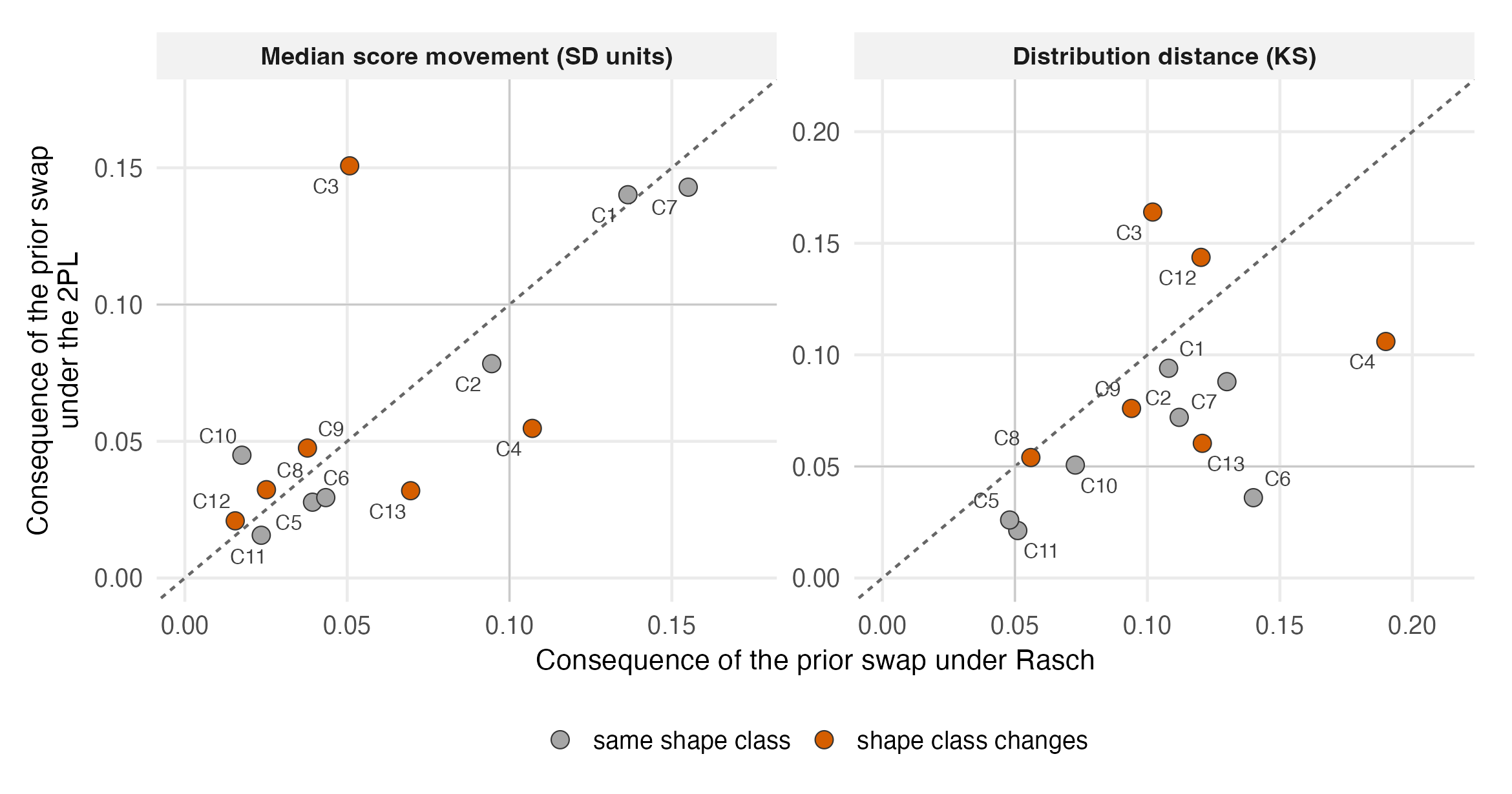
Figure 16.1 compares the prior swap’s consequence on the same data under the two models. The diagonal is not the story; the departures from it are, and they are the flip cases. C3’s individual scores move three times as far under the 2PL as under Rasch (0.151 against 0.051 SD) and cross the materiality bar only there, consistent with its class flip from bimodal to skewed, the score-moving class. C4 runs the other way: its score movement is material only under Rasch (0.107 SD against 0.055), and its between-prior distribution distance halves under the 2PL (KS 0.190 to 0.106) while remaining material as the fitted reliability coordinate also falls. These co-movements do not identify which model component caused the difference. C9’s flip changes the matched roster rather than the consequence: its distribution contrast is material under both models, but only its 2PL row carries a placeable class, bimodal, while its Rasch row is non-normal without one and identifies no simulation cell. The flips are model-conditional heterogeneity, not a demonstrated mechanism.

Figure 16.1: The item model changes how much the prior matters on the same data, and several large disagreements coincide with a change in the standardized shape class. Each point is one case, placed by the size of its prior-swap consequence under Rasch (horizontal) and under the 2PL (vertical); the left panel measures median individual-score movement, the right the KS distance between the two reported distributions; thin grey lines are the materiality thresholds and the dashed line is equality. Orange cases are the six whose standardized shape class differs between item models (C3, C4, C8, C9, C12, C13): C3 moves scores three times as far under the 2PL (0.15 against 0.05 SD) and crosses the score-materiality bar only there, while C4’s score movement is material only under Rasch and its between-prior distribution distance halves under the 2PL (KS 0.19 to 0.11) while remaining material. Choosing the item model is not upstream of the prior question; it is part of it. The coincidence is a description of these thirteen cases and not a causal explanation, and these are consequence measurements: they establish that the choice moves the report, not which item model or prior is closer to the truth. Values from the frozen comparison rowset; classes from the standardized shape manifest.

16.3 The model changes the matched verdict third

Figure 16.2 carries the same comparison into the matched cells: the simulation’s KS loss ratio for each case’s Rasch placement beside its 2PL placement.

Figure 16.2: Every matched non-normal case-cell favors the flexible prior on distribution recovery, and the size of that advantage can differ between the two item models fitted to the same data. For each of the 14 recommendation-eligible non-normal matches, the point gives the simulation’s KS loss ratio (DP-focused + GR against Gaussian + GR) in that case-cell’s matched cell, with its bootstrap interval; blue = the case’s Rasch match, yellow = its 2PL match, glyph = the shape class. C12–Rasch and C4–2PL are absent because their reliability values fall below nearest-tier support. All displayed intervals sit below 1, conditionally on the matched simulation cells; the reliability side of each match is a nearest-tier approximation carrying a gap, so each ratio is read at the tier rather than at the case’s own reliability. Direction here is the simulation’s to establish, and the case supplies only the coordinates at which it is read; ratios come from the current sim-v3 evidence map.

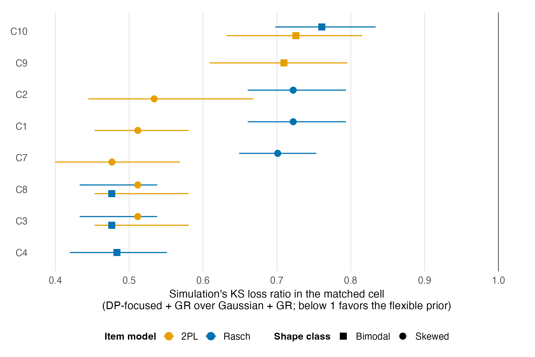
Every displayed non-normal row’s interval sits below parity, so the matched-cell direction does not reverse; what changes is the size of the result (ratios from 0.476 to 0.761 across placements of the same portfolio) and, for the flip cases, the mechanism behind it: C3 is matched to a bimodal cell under Rasch and a skewed cell under the 2PL, so its two placements inherit the two different sides of the simulation’s dissociation. The direction is the simulation’s, read at two different addresses, so the transfer stays conditional on the item model: a case that changes cells changes the verdict it inherits.

16.4 What to do with a disagreement

The portfolio’s honest advice is procedural rather than adjudicative. Fitting both models costs one extra fit per prior and delivers three diagnostics no single-model analysis has: whether the standardized shape class is stable across the two models, whether \bar\rho is stable (C4’s half-point drop under the 2PL is itself a finding about the instrument, a few items doing all the work), and whether the substantive consequence (Part IV’s families) is stable. Where the two models disagree, the disagreement is information about fitted-model sensitivity, not an inconvenience. It does not show that the 2PL “explains away” a true mode or that discrimination estimates caused the flip. The protocol chapter folds this into its steps; the deeper question of which item model is right for a given instrument belongs to the theory volume, not here.