1 Two choices behind every score report
An operational item response analysis produces three kinds of report from one fitted model: a score for each person, an ordering or a selected group, and a distribution, the histogram in the technical appendix, the standard deviation in the norms table, the percentile a raw score is converted into. Figure 1.1 shows all three built from a single real dataset, the grade-3 reading comprehension test that will reappear throughout this book as case C1.
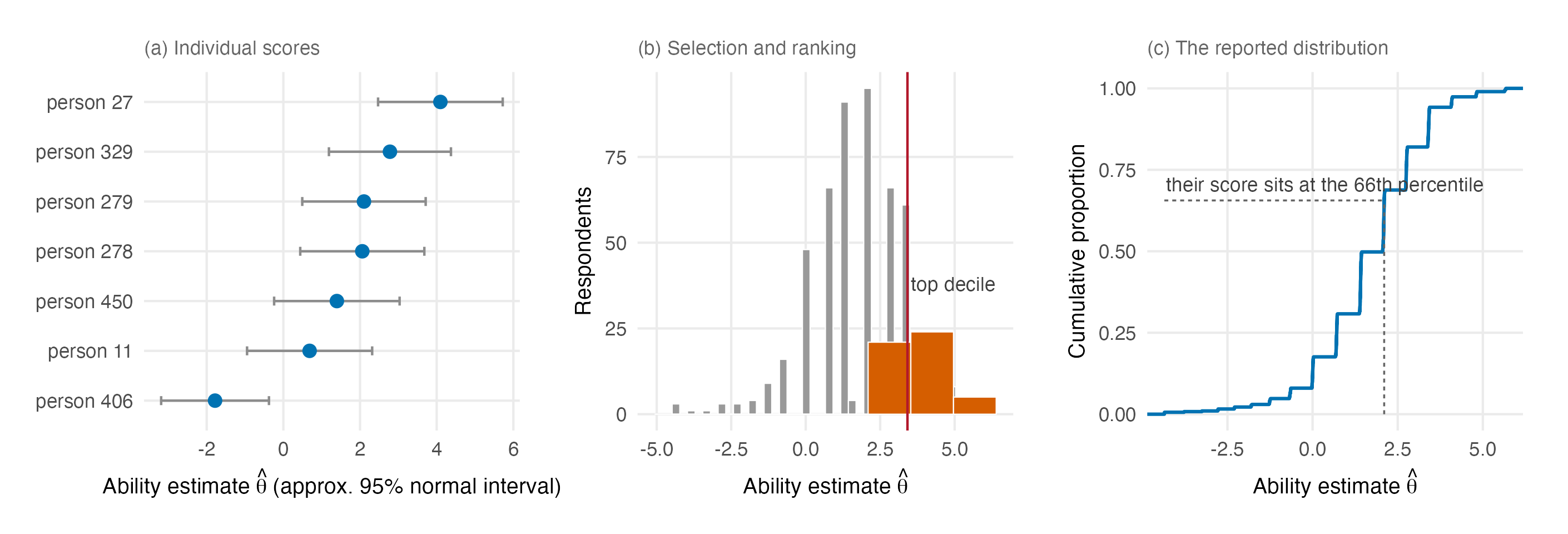
The analysis behind those reports made two choices that most software makes silently. The first is the prior for the latent ability distribution G. The conventional choice is the standard normal, and it is not innocent: with a Gaussian prior, the model will report a roughly Gaussian ability distribution whether or not the population is one, because the prior is part of what the reported distribution is made of. The alternative studied in this project replaces the normal with a Dirichlet process mixture (DPM), which lets the data place probability mass where it finds it, in a shoulder, a second mode, a long tail. It requires heavier computation and introduces two elicitation settings of its own.
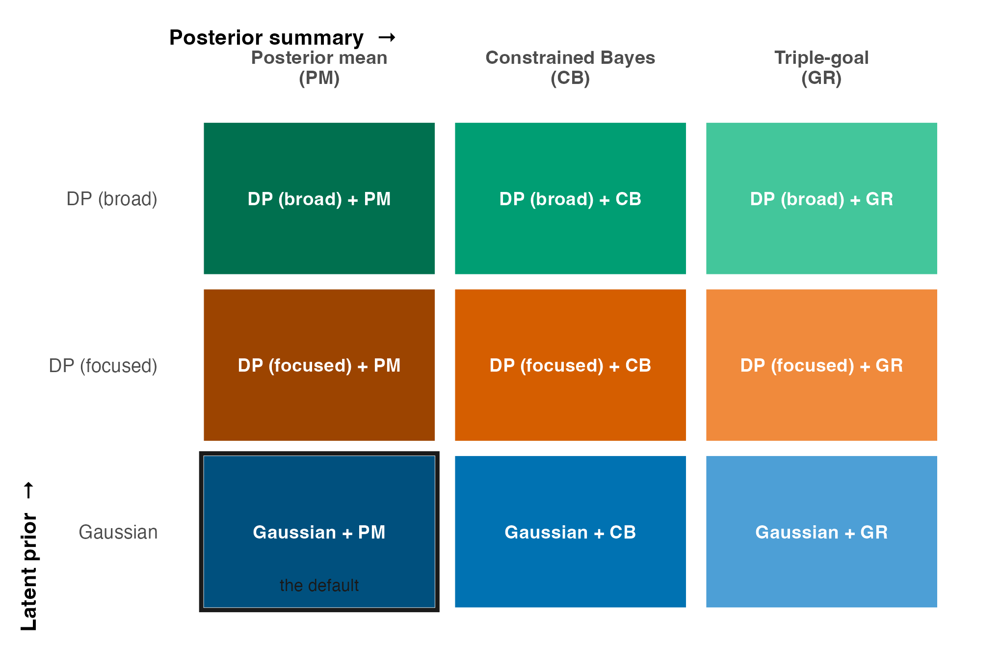
The second choice is the posterior summary: the rule that collapses each person’s posterior distribution into the one number that is reported. The posterior mean (PM) is optimal for each person’s squared error and is what nearly all software reports. It achieves that optimality while shrinking toward the center, so the ensemble of PM estimates is systematically narrower than the population it is meant to describe; a histogram of PM scores understates the spread of ability as a matter of arithmetic, not of misfit. Two established repairs re-aim the summary at the ensemble rather than the person: the constrained Bayes summary of Ghosh (1992) (CB) rescales the estimates so their mean and marginal variance match the corresponding posterior moment target. This implementation is exact under posterior independence; shared item and hyperparameter uncertainty can induce cross-person covariance that it omits. The triple-goal summary of Shen & Louis (1998) (GR) targets the posterior expected finite-sample realized EDF G_N and each person’s posterior expected rank, then assigns EDF quantiles by rank. Neither is exotic; both are a few lines of post-processing on the same fitted model.
Crossing three priors (the Gaussian, a calibrated “focused” DPM, and a deliberately diffuse “broad” DPM) with the three summaries gives the nine combinations of Figure 1.2, and the pair of choices, prior and summary together, is the object this project studies. We refer to the two choices as levers. Their apparent relative length depends on the estimand: the current simulation-wide factorial decomposition assigns more variation to summary, while one-swap comparisons on the exploratory case join need not. Under the registered paired-geometric crossed comparison, Gaussian + GR beats DP-focused + PM in 100 of 120 simulated cells.
1.1 Why real data, and why these
The project’s manuscript originally argued from design descriptors alone: a reader was given a sample size and a reliability, and the simulation’s tables answered for a hypothetical test of that description. The argument was correct and unpersuasive in equal measure, because it never touched an actual dataset, and because two of its inputs, reliability and latent shape, turn out to be measurements with their own error and their own model-dependence rather than known labels. The present volume replaces the hypothetical section with thirteen real tests, selected from the Item Response Warehouse (Domingue et al., 2025) to span the simulation’s grid as far as real dichotomous data allow, each fitted under both item models (Rasch and two-parameter logistic) and all nine combinations, with every comparison frozen before any result was seen.
Real data change the question. In the simulation, truth is known, so the question is which combination recovers it. On a real test no such adjudication is possible, and this book never attempts one. What a real test can establish is consequence: how much the reported output changes when the choice changes, in the quantities a technical report actually prints. The division of labor between consequence and correctness, and the discipline it imposes on the language of this book, is the subject of Chapter 3.
1.2 The plan of the book
The plan of the book is as follows. Chapter 2 compresses the simulation volume’s findings to what a reader of this one needs: the two levers, the reliability gradient, exploratory grid guidance, and the post-outcome safety interpretation. Chapter 3 fixes the epistemic ground rules. Part II introduces the corpus and the portfolio: the screening funnel (Chapter 4), the measurement of a real test’s three coordinates and the two ways it is harder than it looks (Chapter 5), and the thirteen cases themselves (Chapter 6). Part III specifies the comparison: the nine combinations, the four output families with their pre-declared materiality thresholds (Chapter 7), and the computation (Chapter 8). Part IV reports what changes on real tests, beginning with the consequence map (Chapter 9) and continuing through individual scores (Chapter 10), the reported distribution (Chapter 11), rankings and selection (Chapter 12), tails and cut scores (Chapter 13), and the reproducibility of the report itself (Chapter 14). Part V matches each eligible case-cell to the simulation cell its coordinates select and reads out that cell’s verdict (Chapter 15), a join that is exploratory because it was assembled after both source volumes’ results; it then examines the item-model question (Chapter 16) and separates safety scope from the cells that carry no match (Chapter 17). Part VI turns the whole into a protocol for a reader with a test of their own (Chapter 18) and closes with what the thirteen cases settle and what they cannot (Chapter 19).