8  Computation, briefly

The comparison behind this book is 78 production fits (13 cases × 2 item models × 3 priors) plus 78 seed-B replicates, all on one cloud node, with NIMBLE as the sampler. This chapter records what a practitioner would want to know before running the same comparison on their own test; the full record, environment, budgets, seeds, verification checks, is Appendix C.

Figure 8.1: The expensive component is the prior, never the summary: a DP fit takes 15 to 17 times as long as its Gaussian counterpart, and all three summaries are computed from the same fitted draws. Points are the 78 production fits, by wall-clock minutes (log scale) and configuration; vertical bars mark medians (Rasch: 13 minutes Gaussian against 230 DP; 2PL: 15 against 222). The DP computation includes latent-density estimation (16,000 retained draws against 8,000, and per-draw mixture bookkeeping); the summaries add seconds. The production wave cost 222 core-hours and the 78 independent seed-B refits another 142, for 364 core-hours recorded in total, all on one cloud node. NIMBLE runs chains sequentially, so fits, not chains, were parallelized. Times from the frozen fit records.

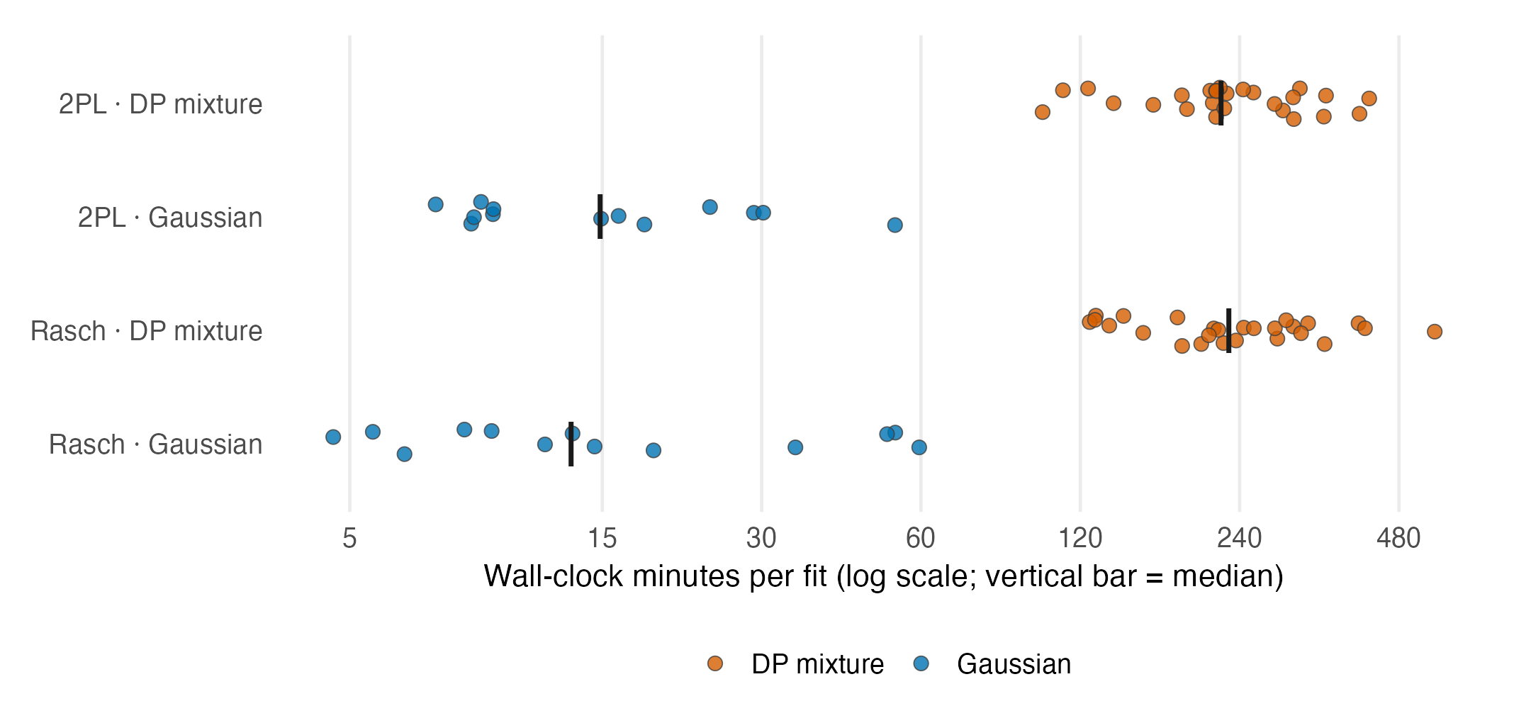
Three facts organize Figure 8.1. The prior is the expensive choice: a DP fit costs 15 to 17 times its Gaussian counterpart at matched specification, which for a 500-person Rasch dataset means roughly 3.8 hours against 13 minutes. The summaries are free by comparison, seconds of post-processing, which is why the simulation’s cheap-fix result (Gaussian + GR) has the practical force it does. And chains run sequentially in this sampler, so the parallel unit is the fit, not the chain: the production wave cost 222 core-hours spread over 78 fits. The independent seed-B audit added 142 core-hours, for 364 core-hours recorded across both waves.

Convergence was monitored on the standard diagnostics, with the two diagnostic axes kept deliberately separate. 4 of the 78 production fits crossed \hat R = 1.1 (worst 1.28, all of them Rasch-DP fits), and they were retained with their diagnostics on record rather than selectively replaced. Across the full audit PM and CB reproduce within 0.028 SD, while GR has the short-form failures documented in Chapter 14. The converse lesson is the important one, and Chapter 14 develops it: a clean \hat R does not certify that a reported summary reproduces, because reproducibility can fail in the summary’s own machinery rather than in the chains. Convergence diagnostics answer a question about the sampler; the seed-replicate design answers a question about the report.

One engineering note that transfers. CB does not use random ranking, and GR consumes random numbers only when rank(rbar, ties.method="random") encounters an exact posterior-rank tie. Exact ties are rare in these stored fits, so random tie-breaking cannot explain the observed GR instability. Every extraction is nevertheless seeded as a reproducibility safeguard; the independent-fit audit remains the relevant test of the report.