5  Three coordinates, measured twice

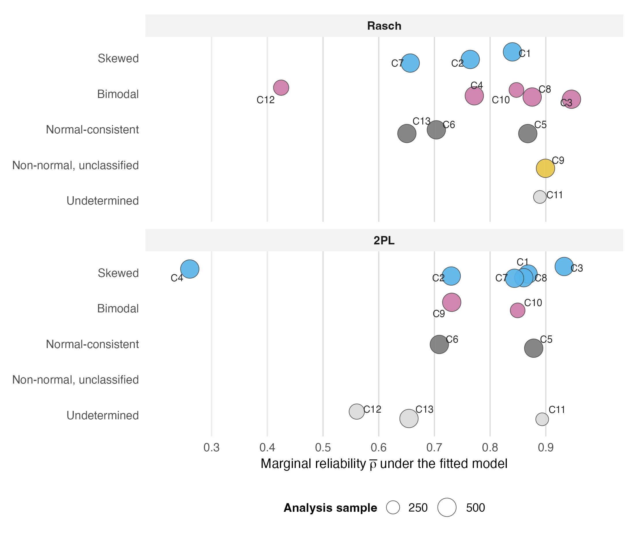
To use the simulation’s answer, a real test must first be located on the simulation’s grid, and the grid has three axes: sample size, reliability, and latent shape. Sample size sounds like the easy one and nearly is; the other two are measurements, made under a model, with error and with model-dependence that turn out to be findings in their own right. This chapter is about the measuring. Its summary, drawn in Figure 5.1, is that a real test does not occupy one exact cell of the grid. Every case has two fitted coordinates, one per item model, and the shape class differs between the two models for six of the thirteen cases. The shape coordinate reported here is the one this edition rebuilt on a standardized statistic (Section 5.4); the reliability coordinate is a fitted-model quantity matched to the grid’s nearest tier, and it carries a gap that no refit removes.

Figure 5.1: A case has no single placement: six of the thirteen change their shape class, and several move a reliability tier, when the item model changes. Each point places one case (labeled C1-C13) on the two coordinates used by the companion simulation: marginal reliability \bar\rho recomputed under the fitted model (horizontal axis; vertical reference lines mark the simulation’s five design tiers) and the standardized shape class (rows, with vertical jitter for legibility). The upper panel shows the 13 Rasch rows, the lower panel the same datasets under 2PL. Point area is the fitted sample: 9 cases at the n = 500 cap, C13 at 497, and three whole corpora of 316, 341 and 235. Undetermined rows mark cases whose design could not have detected a simulation-sized departure of either kind, and one Rasch row holds the single case-cell the standardized screen reports as non-normal without a class (C9). The shape coordinate is validated and of record, while the reliability coordinate is a fitted-model quantity read against a design-time tier, so a horizontal placement is a nearest-tier approximation rather than an exact match. The reliability spread is 0.42 to 0.95 under Rasch.

5.1 Sample size, and the one hard constraint

The design uses two samples per case. Coordinates are measured on a characterization sample of up to 5,000 respondents, which never touches the method comparison; the nine combinations are then fitted to an analysis sample of at most 500, drawn once with a recorded seed. The cap is a package constraint, not a choice: the DPM elicitation routine accepts at most 500 persons, and the elicitation is a function of the analysis sample size. Three small datasets are fitted whole; every large case contributes exactly 500 (C13: 497 after three all-null respondents were dropped at fit time, a detail recorded because the design frame says 500). For grid placement, N matches downward to the nearest simulation value, so a 341-person case reads the N = 200 cell.

5.2 Reliability has no single value

Reliability enters the project twice, as a screening variable from the warehouse and as the placement coordinate, and the first edition of this book planned to treat the two as interchangeable. They are not, and the discrepancy is one of the sharpest methodological findings the portfolio produced. The warehouse’s coefficient is EAP-based (mirt’s marginal_rxx); the simulation’s grid is built on \bar\rho, an inverse-information approximation to mean squared error of measurement, conditional on fitted item parameters. It averages 1/J(\theta) and omits item-calibration and model uncertainty. Both are useful fitted-model functionals, but they do not agree about the portfolio: the median 2PL-minus-Rasch gap is +0.215 under marginal_rxx against +0.004 under \bar\rho, the two coefficients agree in sign for only 6 of 13 cases, and on the vocabulary-checklist case C4 they move in opposite directions by half a scale point each (+0.48 against -0.51) on the same pair of fits. Figure 5.2 displays the disagreement.

Figure 5.2: The two reliability coefficients disagree about which item model is more reliable, and can disagree in sign on the same fits. Each point is one case; the horizontal axis gives the 2PL minus Rasch difference in the warehouse’s EAP-based coefficient (mirt’s marginal_rxx), the vertical axis the same difference in \bar\rho, the MSEM-based functional the simulation grid is built on. Points in the shaded off-diagonal quadrants (orange) are cases where the two coefficients rank the item models in opposite order; the dashed line marks equality. The median gap is +0.215 under marginal_rxx against +0.004 under \bar\rho, the signs agree for 6 of 13 cases, and C4 moves +0.48 under one coefficient and -0.51 under the other on the same pair of fits. Both coefficients are computed from the frozen characterization layer.

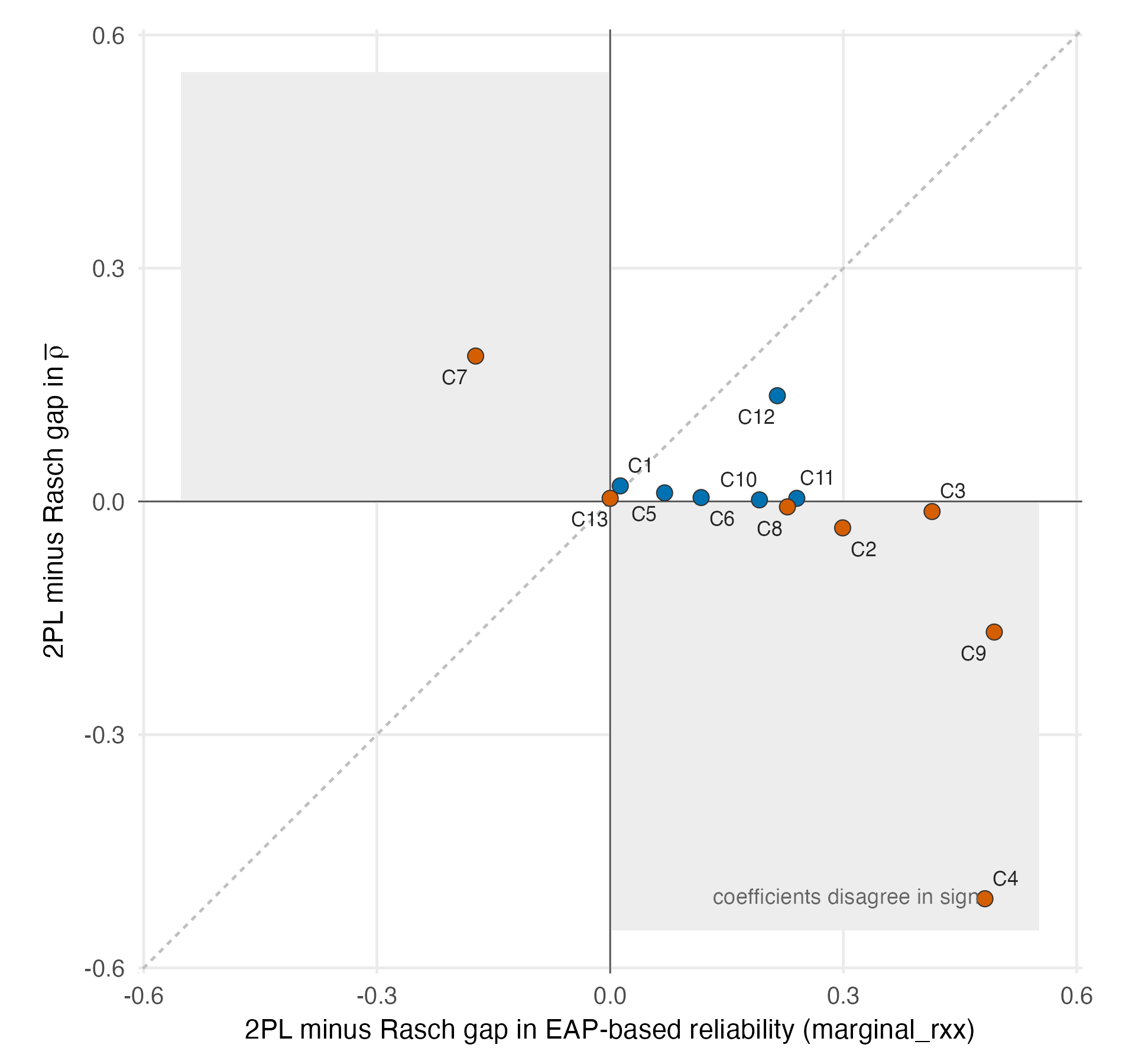
The lesson is not that one coefficient is wrong. The EAP-based coefficient answers a question about score precision under the fitted scoring rule; the inverse-information approximation answers a question about information against the latent metric, and a 2PL that concentrates its discrimination on a few items can raise the first while lowering the second. The lesson is operational: “the test’s reliability” is underdetermined until the functional is named, and a reader placing their own test on the simulation’s grid must compute the grid’s own functional, \bar\rho, under the model they intend to fit. The warehouse coefficient screened this corpus; it places nothing.

5.3 Shape cannot be read off a small sample

Latent shape is the coordinate the whole flexible-prior question turns on, and it is the one that cannot be read safely from a small sample. A naive fixed-threshold screen flagged 47 of 54 small warehouse datasets under the 2PL and 22 under Rasch. Truth is unknown in those real datasets, so these are not measured false-positive rates. They instead show that the naive flag is strongly model-dependent and likely contaminated by finite-design artifacts. Figure 5.3 shows the relevant behavior under known normality.

Figure 5.3: A design-matched null is not optional at these sample sizes: on data whose latent trait is exactly normal, the dip statistic still flags multimodality in most replicates at n = 100. Curves give, for simulated datasets whose latent trait is exactly normal, the median KS distance of the recovered density from the normal (left) and the share of null replicates whose dip statistic flags multimodality (right), by respondents (horizontal, log scale) and items (color). At n = 100 the dip flags multimodality in about 98% of perfectly normal replicates regardless of test length, falling to 44% at n = 350, 32% at n = 500 and near zero only by n = 1,500; the KS floor falls with items as well as respondents. Any shape label assigned to a small dataset without such a calibration mostly measures the procedure, not the population. This design sweep sets the general expectation and is not the authority for any case’s class; each class of record is decided against that case’s own standardized null band. Values from the frozen null-calibration table (200 replicates per design point), computed under the earlier native-scale jitter.

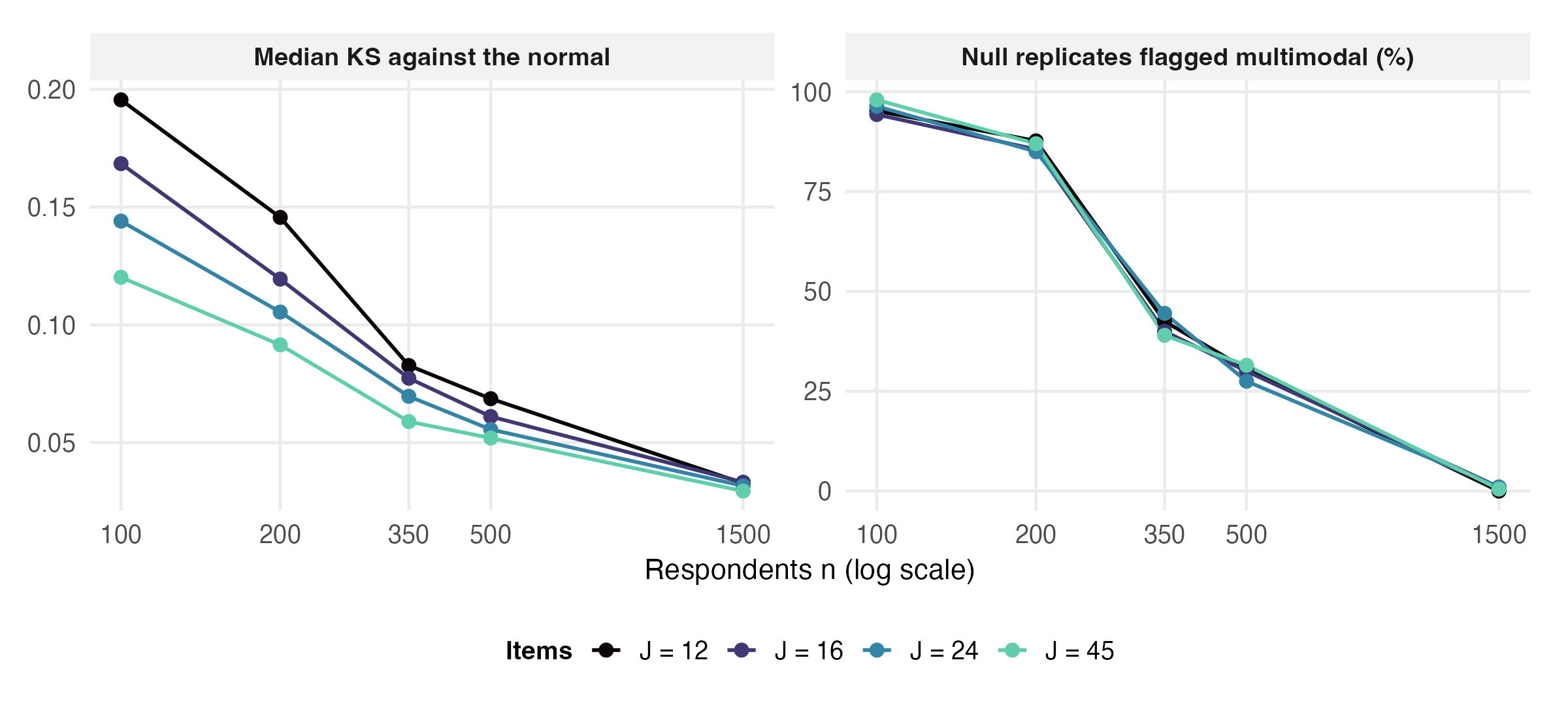
The screen calibrates a null per case: two hundred refits of data simulated from a normal population with the case’s own n, item count and item parameters, giving each statistic its own 95th percentile under normality for exactly this design. A case earns a class only by exceeding that null and by reaching at least half the simulation condition’s departure, so the class means “departs, and by enough for the simulation’s cells to speak to it”. The classifier has two further branches that matter and that the first two editions of this book failed to describe. Between a quarter and a half of the condition it returns mild-skewed or mild-bimodal. And it asserts normal only when this design’s nulls are tight enough that a condition-sized departure of either kind would have been detected; otherwise it returns undetermined, because “not flagged” and “normal” are not synonyms.

5.4 The statistic that had to be rebuilt

An external audit of the previous edition found a load-bearing defect in one of the three statistics. The dip was computed by resampling from the fitted density and adding jitter of 0.05 on each fit’s native scale, and the fitted density’s standard deviation ranges from 0.51 to 2.15 across the 26 case-cells. The smoothing was therefore between 2.3% and 9.7% of a standard deviation depending on the case, and the case’s statistic, its own null (generated at the Gaussian fit’s scale) and the simulation’s reference condition (computed on standardized draws) were three mutually incompatible quantities. Skewness, excess kurtosis and the KS distance were never affected: they are computed analytically from the density weights as standardized moments, so they are scale-invariant by construction. The defect was confined to the dip.

Because the fitted supports and weights behind the original null draws had not been retained, the repair required refitting rather than recomputation. This edition ran it: 26 observed empirical-histogram refits and 5,158 retained null replicates of 5,200 attempted, reproducing the original fits exactly – same characterization samples, same convergence ladder, same seed tree – and changing one thing. The dip is now computed by the published ancestor’s procedure, which standardizes the weighted support to mean zero and unit variance and then jitters on that scale, and the same estimator is applied to the observed densities, to every null replicate and to the simulation’s reference conditions.

Two checks establish that the refit is faithful and that the repair is the only thing that moved. The scale-invariant statistics reproduce the frozen values to within 0.00018 in skewness on 24 of the 26 cells. The two that move further are numerically borderline density fits rather than disagreements about the data: C12–Rasch, which needs the 8,000-cycle rung of the convergence ladder, lands 0.064 away, and C9–Rasch, at the portfolio’s largest fitted spread, lands 0.005 away. The reference condition’s dip, in turn, is 0.054 unjittered against 0.054 under the standardized estimator, so the jitter asymmetry the audit flagged in the half-condition gate was immaterial in size.

The labels themselves barely moved. Exactly 1 of 26 changes: C9–Rasch, which the previous screen left undetermined, now reaches the KS branch and is reported as non-normal without a class. That single change is not attributable to the standardization. Running the old native-scale estimator through the same machinery reproduces 25 of the 26 frozen labels and moves C9–Rasch in the same direction, so what moved it is the refit variation of a borderline fit. All nine skewed, all seven bimodal and all five normal-consistent labels stand under both estimators.

The correction was necessary and its consequence for the portfolio is nearly nil, which is the most useful outcome a repair of this kind can have. The shape coordinate is now measured on a standard commensurable with its own null and with the simulation grid it is matched to, and everything the previous editions reported by shape class survives intact.

One inference the repair does not license is worth stating, because it was our own first expectation. The dip’s correlation with the fitted latent standard deviation falls only from 0.59 to 0.54. Standardization removes the incomparability between a statistic and its reference; it does not remove the association between bimodality and variance, and most of that association is signal rather than artifact, since a population with two separated modes genuinely has a larger variance.

Figure 5.4: Every shape call is made against a null built for that case’s own design, and on the standardized statistic 22 of the 26 case-cells earn a determinate class, 21 of them in a class the simulation’s grid contains. For each case (columns within panels) the grey bar spans from zero to the 95th percentile of that case’s own null calibration (200 refits of normal data at the case’s n, item count and item parameters); the point is the observed value, upward-filled when it exceeds the null and downward when it does not. Dashed lines mark half the simulation condition’s value (skewness 1.43, dip 0.054), the second requirement a class must meet. Fill gives the class of record. Every quantity plotted here is the standardized one that actually set the class: the dip and its null come from the observed-and-null refit, the reference conditions are recomputed by the same estimator, and skewness is scale-invariant, so its standardized and frozen values coincide. C12’s Rasch dip (0.099) is the portfolio’s largest. Standardized shape manifest and null band; 200 null refits per case-cell, of which 176 to 200 converged.

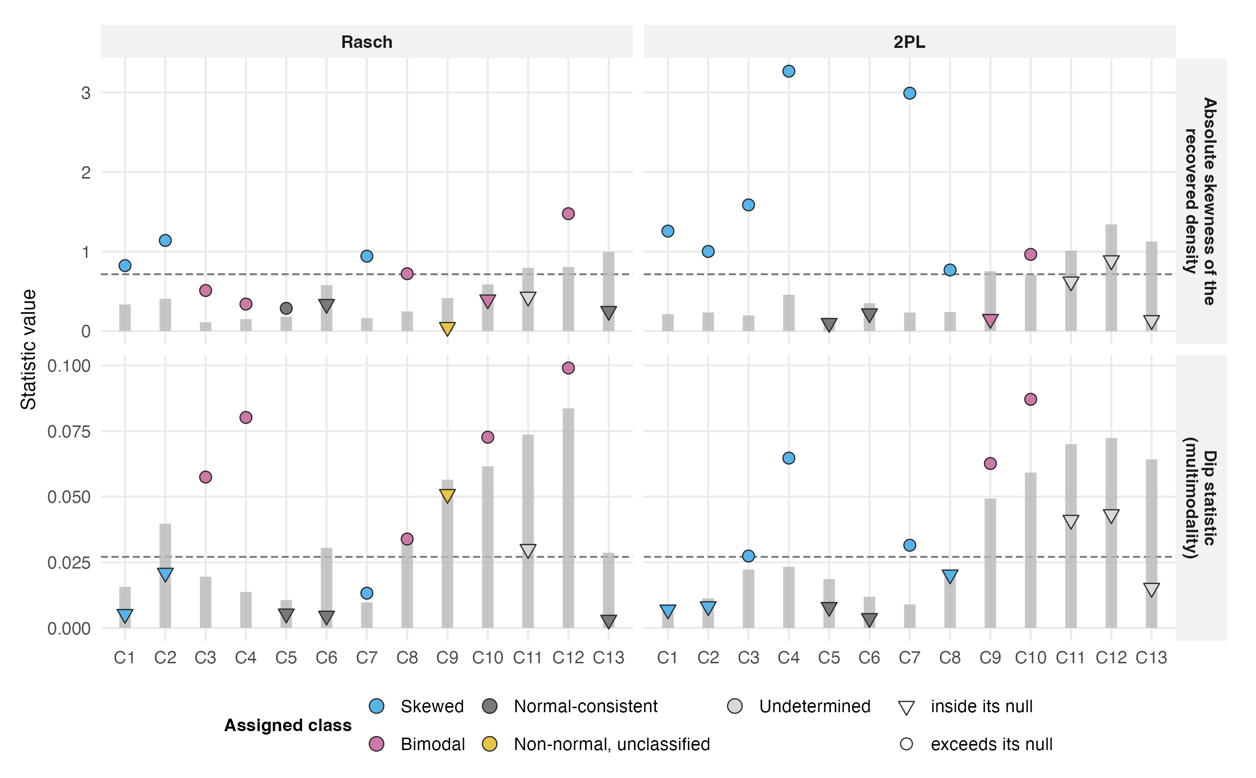
Two safeguards in the screen are worth carrying into practice, and neither would have repaired a statistic computed on inconsistent scales: require both design-specific evidence and a departure of practically comparable magnitude, and read skew, dip and KS jointly rather than separately.

5.5 Reliability-tier placement and the freeze

The continuous fitted \bar\rho values and analysis seeds were frozen before the production fits. The first edition then discretized reliability to the nearest tier but silently mapped every value below .55 to .5. C12–Rasch (\bar\rho=.425) and C4–2PL (\bar\rho=.261) lie below the .5 tier’s nearest-cell support boundary of .45; their former .5 matches are removed, and this edition reports for every row the continuous coordinate, its nearest tier, the absolute gap and the support status.

That leaves 19 rows carrying both a validated shape class and a reliability inside the grid’s support. Those rows are matched to simulation cells in Chapter 15. The reliability side of the match remains an approximation and is the weaker of the two coordinates: the case’s \bar\rho is a fitted-model quantity computed on real responses, while the grid’s tier is a design-time quantity computed on known generating parameters, and the two are commensurable in definition rather than identical in construction. Every matched row is therefore reported with its tier gap, which reaches 0.049 at worst.