11  The reported distribution

The second family is the ensemble-level report: the histogram in the appendix, the SD in the norms table, the curve a percentile is read off. It is the family the flexible prior exists to serve, and on these cases it is where the prior’s consequence concentrates, with a twist that the score results make sharp: the distribution moves most exactly where scores move least.

11.1 Materiality inverts between families

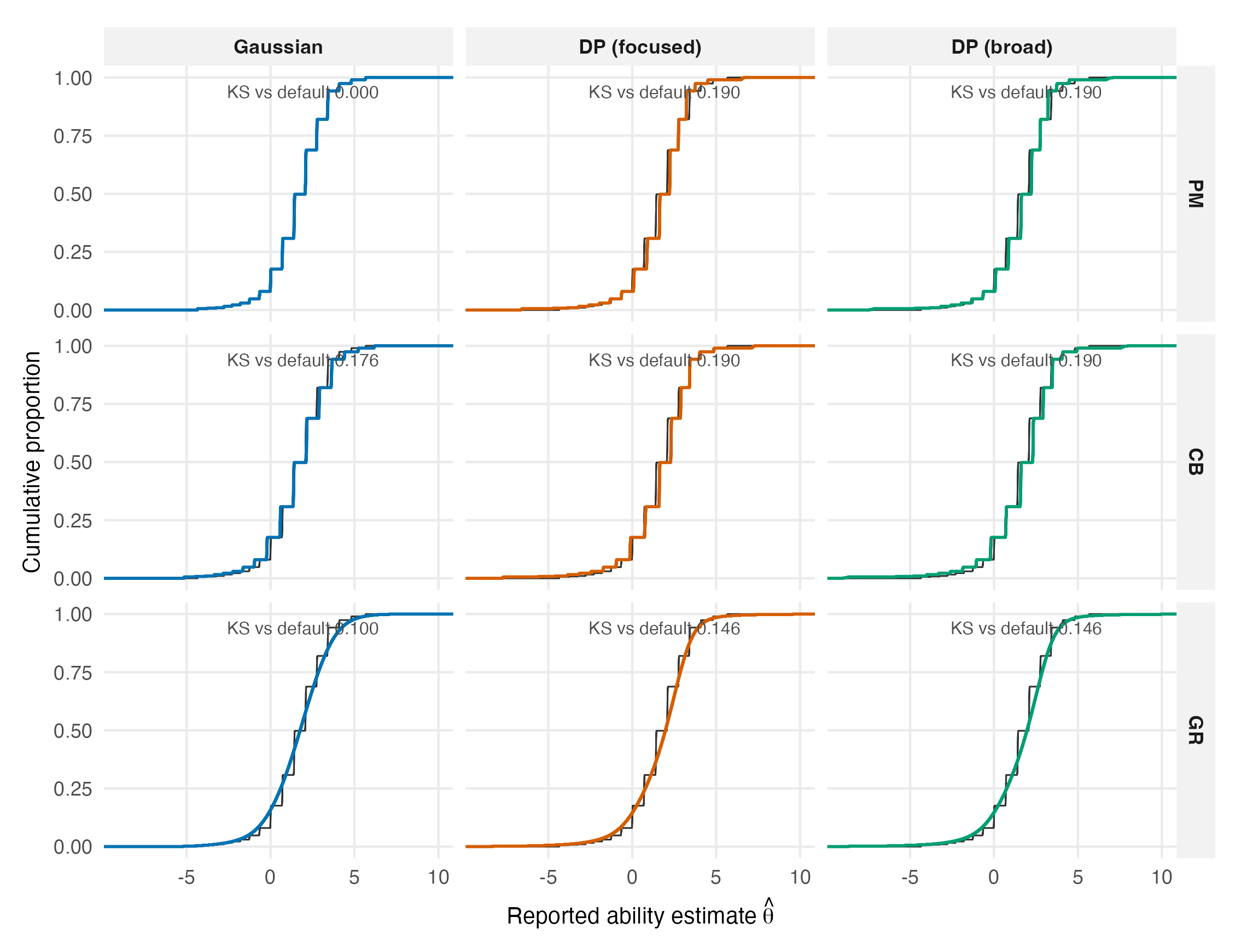
Of the seven bimodal case-cells, one was material on individual scores; on the reported distribution, all seven are, with a median between-prior KS of 0.076. The skewed cells are material nine of nine (median KS 0.106), the normal controls two of five with a median at 0.048 against the 0.05 bar, controls behaving as controls. Under bimodality, then, the prior changes the reported distribution without moving the people in it. A reader who checked a handful of individual scores, found them unchanged, and concluded the prior did not matter would be wrong about the norms table they were about to publish; Figure 11.1 shows the phenomenon on C4 directly, with the summary swap beside it for scale (on this family the two levers are both material almost everywhere, and which displaces the curve farther is the reliability-governed question Chapter 9 settled).

Figure 11.1: One real dataset, nine reportable distributions: the summary decides the family of the curve, the prior decides its details, and the default sits in the corner as one choice among nine. Each panel shows the empirical distribution function of one prior + summary combination’s reported estimates for the conspiracy-beliefs case under the Rasch model (C4, 16 items, n = 500, bimodal placement, reliability 0.77); the thin black curve repeated in every panel is the default report (Gaussian + PM), and the printed value is the KS distance between the panel’s estimate set and that default. Reading down a column shows the summary swap (PM’s clumped staircase, CB’s rescaled version, GR’s full-range curve); reading across a row shows the prior swap at a fixed summary. Estimates from the frozen run store, seed A.

11.2 A family change, not a rescale

The moments of the reported ensembles say what kind of change this is, and they say it only if read together. On the skewed cells the DP arm’s ensemble has a larger standard deviation (ratio 1.064) and a smaller interquartile range (ratio 0.925), and its excess kurtosis moves from -0.17 under the Gaussian to +1.14. More spread overall, less spread in the middle, is not a rescaling; it is one distribution family being replaced by another, a platykurtic shrunken ensemble giving way to a leptokurtic one with a tight core and heavy tails. The bimodal cells show the same signature more weakly in spread (SD ratio 1.031, IQR ratio 0.994) and clearly in shape (kurtosis -0.04 to +0.77). Figure 11.2 places every case-cell on this plane.

Figure 11.2: The prior swap replaces one distribution family with another rather than rescaling: on the skewed cells the ensemble’s standard deviation rises while its interquartile range falls. Each point is a case-cell, placed by the DP-to-Gaussian ratio of the reported ensemble’s SD (horizontal) and of its IQR (vertical); a pure rescaling would sit on the dashed diagonal, and points in the shaded quadrant are wider by one measure of spread and narrower by the other. Point area gives the absolute change in excess kurtosis; white diamonds mark the frozen class-level values (skewed: SD ratio 1.064, IQR ratio 0.925, excess kurtosis -0.17 under the Gaussian prior to +1.14 under the DP). A norms table built from these estimates inherits whichever half of this signature the analyst’s single spread statistic happens to measure. Ratios from the frozen comparison rowset (prior contrast, PM summary).

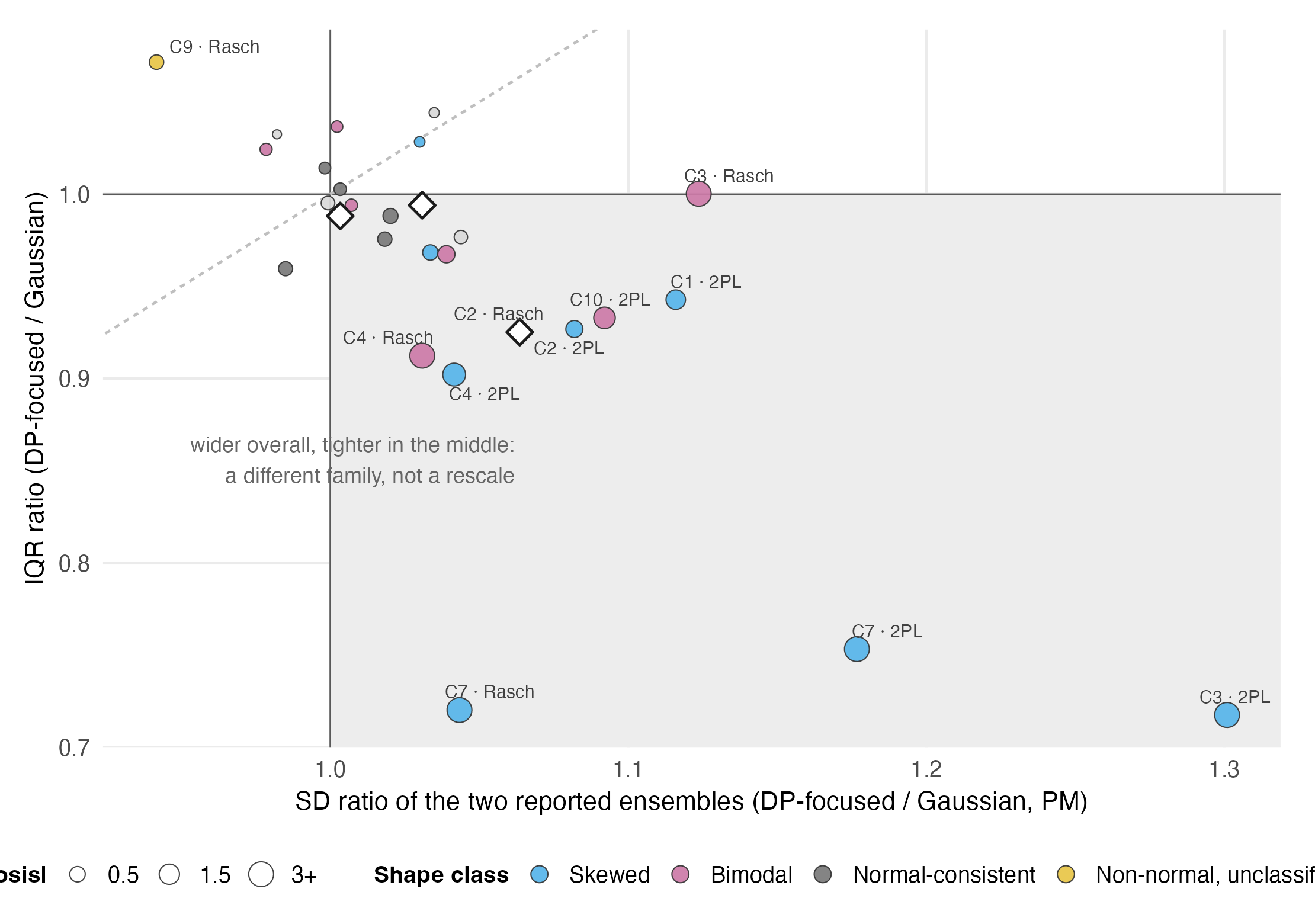
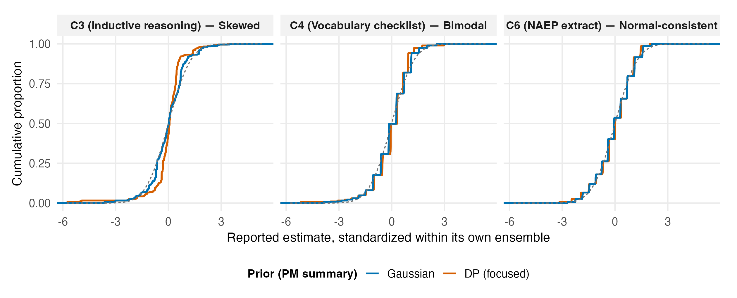
Had this book reported only the SD ratio, the finding would read “the DP prior disperses the ensemble by about 6%”; only the IQR ratio, “the DP prior tightens the ensemble by about 8%”. Both sentences are true and neither is the finding, which is why the comparison layer refuses to collapse F2 to any single spread statistic, and why it refused from the start to standardize the outputs before comparing them: a standardizing step sets the SD ratio to one by construction and would have converted this signature into an artifact pointing the wrong way. Figure 11.3 runs the check the refusal implies: after standardizing each ensemble within itself, the two priors’ curves still separate on the non-normal cases and coincide on the control. What remains after location and scale are removed is the part no affine correction can supply.

Figure 11.3: Standardizing each ensemble to mean zero and unit variance removes every location and scale difference, and the two priors’ reported distributions still disagree where the population is non-normal. Curves are the EDFs of the default-summary (PM) estimates under the Gaussian and DP-focused priors, each standardized within its own ensemble, for a skewed case (C3 under 2PL), a bimodal case (C4 under Rasch) and a normal control (C6 under Rasch); the dashed curve is the standard normal reference. What remains after standardization is exactly what a variance-matching correction cannot repair: the family of the curve. On C6 the two priors coincide; on C3 and C4 they part in the shoulders and tails. These examples are drawn from cases whose person-level derived estimates may be redistributed. Estimates from the permissive-case frozen run store, seed A.

11.3 What the flexible prior estimated

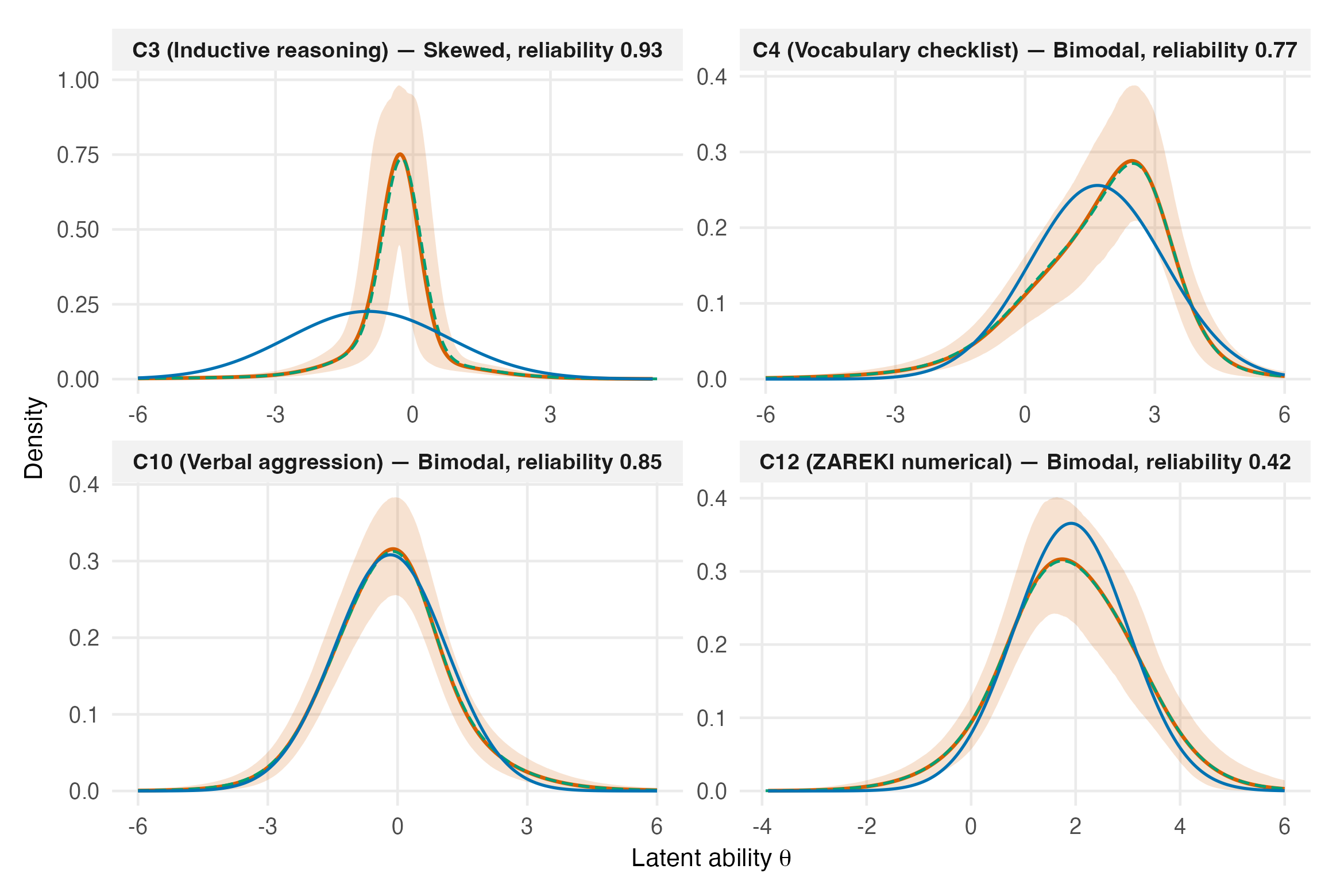
The reported ensembles are summaries; the object the DP arm actually estimates is the latent density itself, with uncertainty. Figure 11.4 shows it for four focal cases with pointwise 95% bands, and it earns a caution the first edition relegated to a footnote. The display is deliberately non-like-for-like: the DP line is a posterior latent-density estimate, whereas the Gaussian reference is a normal curve fitted to the shrunken Gaussian-PM ensemble. It illustrates a reporting contrast, not a density-estimator contest. The DP curve is a posterior mean over 16,000 draws, and averaging smooths: a population the shape screen classifies as bimodal from its score pattern can present a unimodal posterior-mean density (C4’s shoulder is visible, C10’s valley shallow), so the panel illustrates what the prior learned, not the coordinate of record. On C12 the band is wide and the flexible density hugs the Gaussian’s: at reliability .43 the data cannot tell the prior much either way, a picture worth holding until Chapter 17.

Figure 11.4: What the flexible prior actually estimates: the posterior latent density with its pointwise 95% band, alongside a different object—the normal curve fitted to the Gaussian arm’s PM ensemble. This is an interpretive overlay, not a like-for-like density-estimator contest. Orange curves give the DP-focused arm’s posterior-mean latent density with its credible band (shaded); dashed green the DP-broad arm’s posterior mean; blue the normal density implied by the Gaussian arm’s PM ensemble (its mean and SD). Four permissively licensed case-cells: the skewed inductive-reasoning case C3 under 2PL (a shoulder the normal cannot represent), the bimodal conspiracy case C4 under Rasch, the bimodal verbal-aggression case C10 under Rasch, and the low-reliability ZAREKI case C12 under Rasch, where the posterior band is wide and the two priors nearly agree: at reliability .43 the data cannot tell the prior much either way. A posterior-mean density can smooth away modes, and the shape screen decides a class from a different statistic against that case’s own null; a unimodal orange curve therefore neither confirms nor refutes the bimodal class a case-cell carries. For display, the cached curves trim grid points below 0.1% of each posterior mean’s peak; across 52 bundles the largest omitted integrated area was 0.143% and no local mode was removed. Densities from the frozen draw-level density store (16,000 retained draws per DP fit).

11.4 What this family establishes

The prior’s consequence concentrates in the reported distribution, and under bimodality it appears there while scores hold still: whether the prior “matters” has no dataset-level answer, only a family-level one. The change is a family change (SD up, IQR down, kurtosis through zero) that any single spread statistic misreports in one direction or the other. Percentile tables and norms built from these ensembles differ between priors even where every individual’s score agrees to two decimals. What this family does not establish, on any case, is which reported distribution is closer to truth. Part V reads the simulation’s answer at the cells these tests occupy, under a join that is exploratory because it was assembled after both source volumes’ results; the direction it reports is the simulation’s, never the case’s.