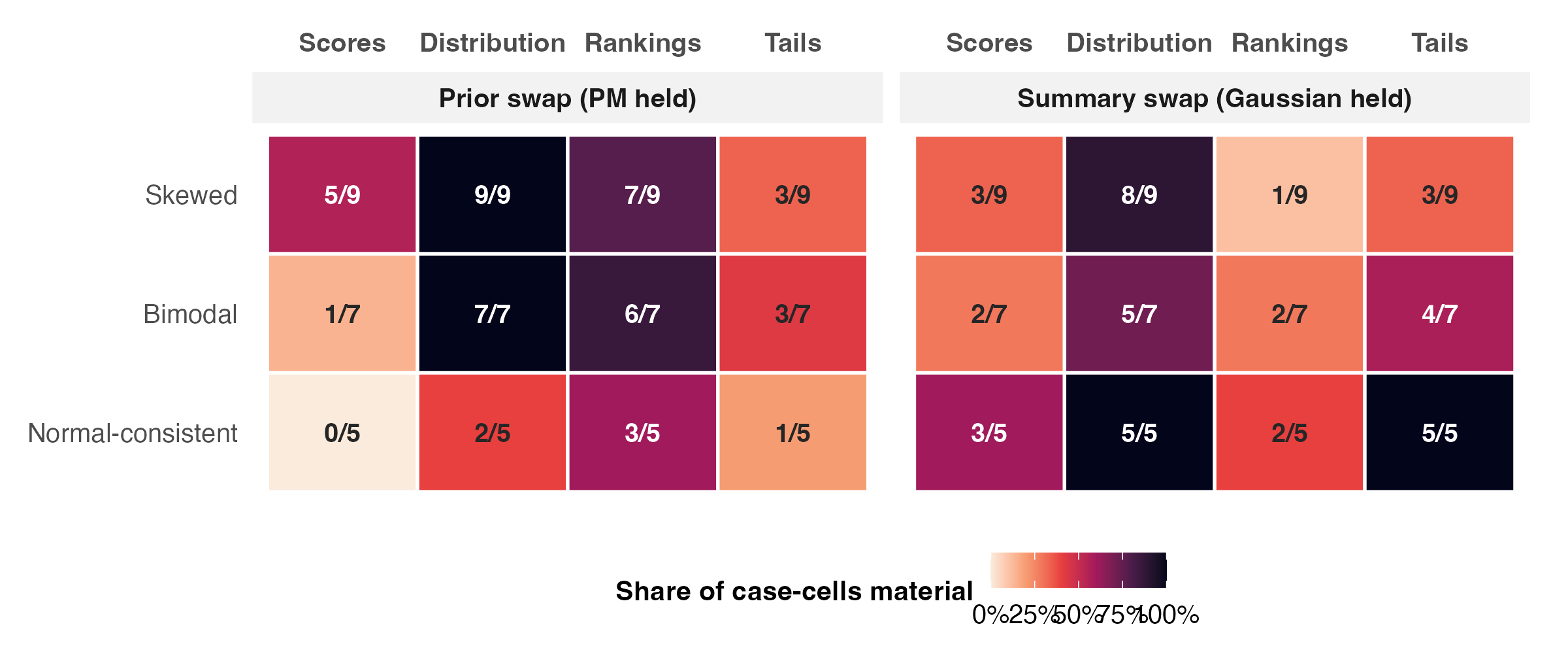
| Shape class | Case-cells | Scores | Distribution | Rankings | Tails |
|---|---|---|---|---|---|
| bimodal | 7 | 1 | 7 | 6 | 3 |
| normal | 5 | 0 | 2 | 3 | 1 |
| skewed | 9 | 5 | 9 | 7 | 3 |
9 The consequence map
Part IV reports what actually changes on the thirteen tests when the two choices change. This chapter gives the whole answer at once, in one display, before the family-by-family chapters take it apart, because the shape of the whole is itself the book’s organizing result: whether a choice “matters” is a property of the output family being reported and of the lever being pulled, before it is a property of the dataset.
All shape-conditioned rows in Part IV group the case-cells by the standardized shape class of Section 5.4. The grouping is descriptive: it says where the portfolio’s departures from normality were measured, not which report is closer to truth.
9.1 Both levers, all cases, all families
Figure 9.1 shows every case-cell (rows), every output family (columns), and both levers (panels), with each change expressed as a multiple of its family’s pre-declared materiality threshold.
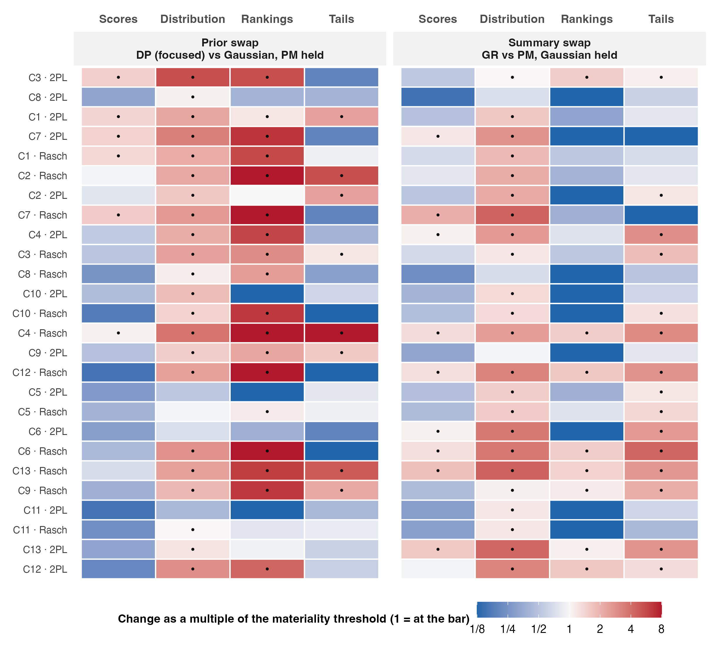
Reading the left panel down its columns gives the prior swap’s geography. On individual scores the red is confined to the skewed rows; on the reported distribution it extends through the skewed and bimodal rows and touches the intended normal-control rows only lightly; on rankings it is strongest exactly where scores are quiet (the bimodal rows, a dissociation Chapter 12 explains); on tails most cells are blue. The localized red cells, and especially the two largest exceptions, are traced in Chapter 13 to mass near a cut and dense bands rather than to a general tail effect. The materiality counts are tabulated in Table 9.1: of the seven bimodal cells, one is material on scores and seven on the distribution; of the nine skewed cells, five and nine.
The right panel is the contrast the first edition of this book specified, froze two claims about, and then never displayed: the summary swap. Its geography is different in both directions. It reaches the distribution family almost everywhere, including the normal controls, because shrinkage repair is not a non-normality phenomenon; and it leaves rankings largely blue, because an affine rescaling (CB) cannot reorder anyone and GR’s reordering is concentrated in dense near-rank bands. The two panels together are the simulation’s two-lever anatomy (Chapter 2), photographed on real data.
9.2 The two levers compared, cell by cell
Figure 9.3 sharpens the comparison to one point per case-cell: the size of the summary swap against the size of the prior swap, for scores and for the distribution. It also forces a distinction the rest of the book depends on, between displacement (how far a swap moves the report) and improvement (how much closer the report gets to the truth), of which a case can measure only the first.
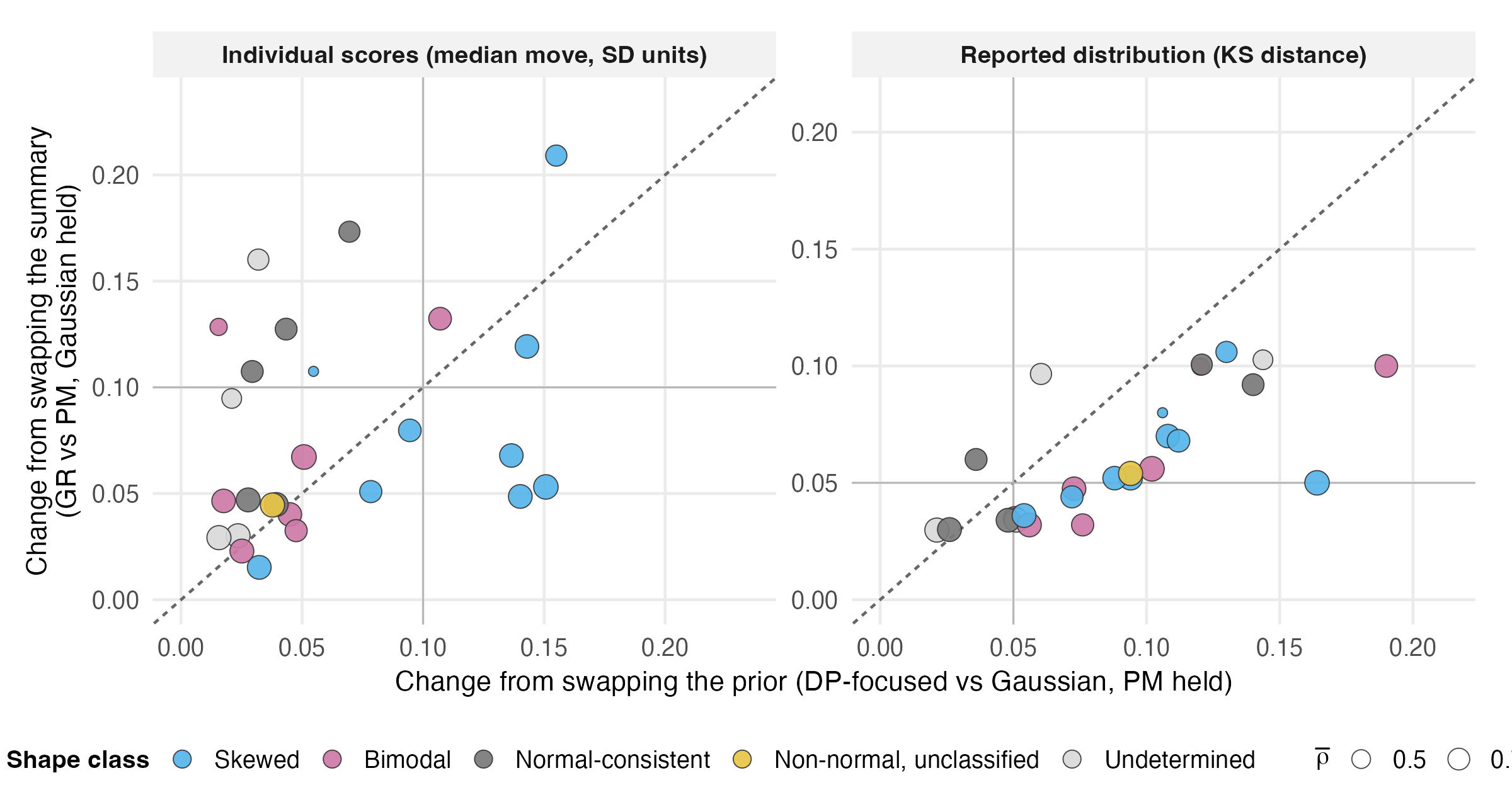
For individual scores the levers divide the portfolio cleanly: on every normal-consistent and undetermined cell the summary swap displaces scores more than the prior swap, and on seven of the nine skewed cells the prior swap displaces them more, which is where the simulation locates the flexible prior’s individual-level action. For the reported curve the ordering reverses: the prior swap produces the larger between-report distance on all sixteen skewed and bimodal cells. Both levers clear the distribution family’s materiality bar on most of the portfolio (the summary swap on 23 of 26 cells, largely through its spread repair), so the reversal is about which material change is larger, not about either being quiet.
The reversal is not a contradiction of the simulation’s larger-lever result; it is that result’s own moderator doing its work. The frozen claims the first edition never presented say how: the summary swap’s size tracks reliability (correlation -0.59 across cells, median movement 0.118 SD below reliability .70 falling to 0.044 above .90; claim C-08), and this portfolio lives at the high-reliability end, where shrinkage, the thing the summary repairs, is smallest. At fixed reliability the summary swap is largest on the normal-consistent cells (0.124 SD against 0.081 skewed and 0.069 bimodal in the .65–.80 band; claim C-09, a blueprint reversal), with a clean mechanism: on a non-normal case the flexible prior supplies part of the spread-and-shape repair on its own, so the summary has less left to do; on a normal case the summary is the only repair there is. The improvement direction cannot be read from these axes. The exploratory sim-v3 join in Chapter 15 compares truth-based losses, but it does not support a universal larger-share claim for the summary on these rows: the answer changes with the factorial, condition-mean, or paired-geometric estimand. How much movement is toward truth is the simulation’s question, not the case data’s.
9.3 The menu against the default
The last display answers the practitioner’s literal question, K1: not “prior versus summary” but “any of the eight alternatives versus what my software already does”.
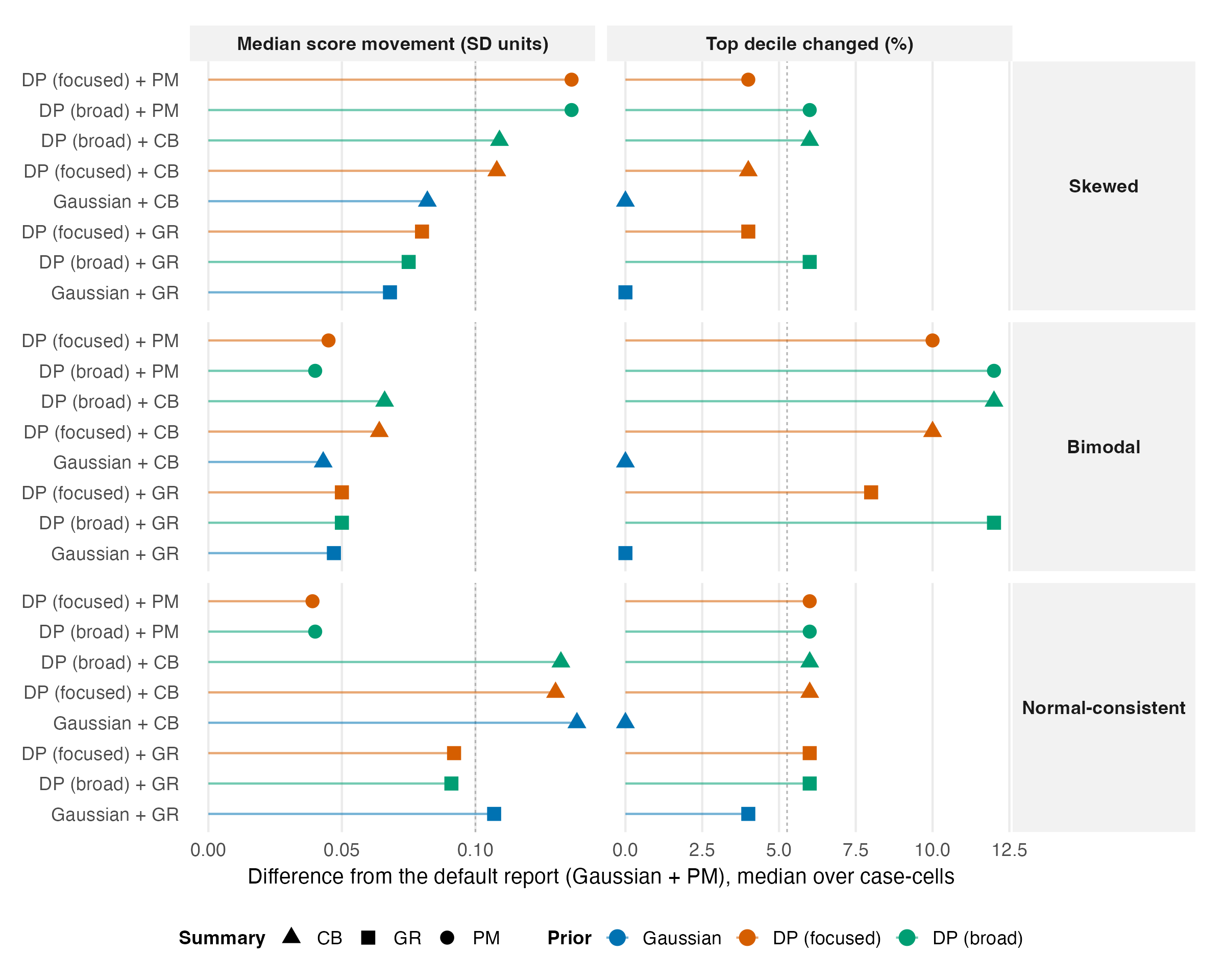
Three readings of Figure 9.4 matter for what follows. On the normal-consistent cases the summary rows dwarf the prior rows: a reader who moves from Gaussian + PM to Gaussian + CB has changed their reported scores by a median 0.14 SD while a pure prior swap changes them by 0.04. Under skew the prior swap joins the summaries in materiality, and the combined swap (DP + GR) is not the sum of its parts. And the right column shows that almost any departure from the default disturbs a top decile by an amount comparable to the paired seed comparison, a warning Chapter 12 makes precise. The family chapters now take the columns of Figure 9.1 one at a time.