15  Each case, matched and judged

Part IV established consequence: the choices change real reports, by measured amounts, in family-specific patterns. This chapter adds the register the cases cannot supply. For each eligible case-cell, its coordinates select one cell of the simulation’s grid, and this chapter reads out what the simulation, where truth is known, concluded in that cell: which combination wins each inferential goal, by how much, and at what price to the goals it does not serve. Every sentence here is the simulation’s, transported; the cases contribute their location and nothing else.

The previous edition could not do this. Its shape coordinate rested on a statistic computed on an incommensurable scale (Section 5.4), so it carried the same join as an explicitly unvalidated sensitivity calculation and issued no case recommendations. The standardized refit has since closed that residual, and the labels it returns are, with one borderline exception, the labels the earlier editions used. What follows is therefore the same arithmetic the previous edition performed, now resting on a shape coordinate that has been validated rather than assumed.

15.1 The roster

Of 26 case-cells, 22 carry a determinate standardized shape class. Two of them, C12–Rasch (\bar\rho=.425) and C4–2PL (\bar\rho=.261), fall below the .5 tier’s nearest support boundary and are removed rather than clamped, leaving 19 eligible rows over 14 distinct simulation cells. Every row carries its continuous reliability, its nearest tier and the gap between them, which reaches 0.049 at worst and 0.033 at the median. That gap is the honest residual of this chapter: the shape coordinate is now measured on the simulation’s own standard, while the reliability coordinate is a fitted-model quantity matched to a design-time tier, and no refit can make those two constructions identical.

The simulation evidence is rebuilt directly from the current volume’s evidence.rds rather than copied from the first edition’s transfer table. On the primary distribution-recovery contrast, 14 of the 19 rows carry a strong_win label, with condition-mean loss ratios from 0.476 to 0.761. Five normal-consistent rows carry harm_flag labels close to parity (0.988 to 1.041), which is imprecision around nothing rather than harm: those are the calibration controls, seen from the case side.

15.2 Winners by goal

Figure 15.1 shows the six-combination condition-mean winner for four goals. A washed tile means the winner is within Monte Carlo error of its runner-up, so on the ranking column, where almost every tile is washed, the winner’s identity is descriptive rather than decisive. The case join adds a second layer of uncertainty on top of that, from the tier gap in the reliability coordinate.

Figure 15.1: Across the 19 matched case-cells, a GR combination wins the distribution goal in 18 of them and a PM combination wins the individual-score goal in 19. Each row is one recommendation-eligible case-cell (ordered by standardized shape class, then by reliability within class); each column an inferential goal; the tile shows the prior + summary combination with the smallest condition-mean loss in that case-cell’s matched simulation cell, on the simulation’s six-combination roster (tile color = prior, glyph = summary). Washed-out tiles are winners within Monte Carlo error of their runner-up, so the identity of the winner there is descriptive; on the ranking goal essentially every cell is such a near-tie, the simulation’s rank-flatness result. The shape coordinate is the standardized one and is of record; the reliability coordinate is a fitted rho-bar read against the nearest design tier, an approximation that every row carries as its tier gap. C4–2PL and C12–Rasch fall below that support and are absent. Each winner is a simulation result read at the matched cell: the case data establish that the choice has consequences, and only the simulation establishes which direction is better. Winners from the current sim-v3 condition-mean store.

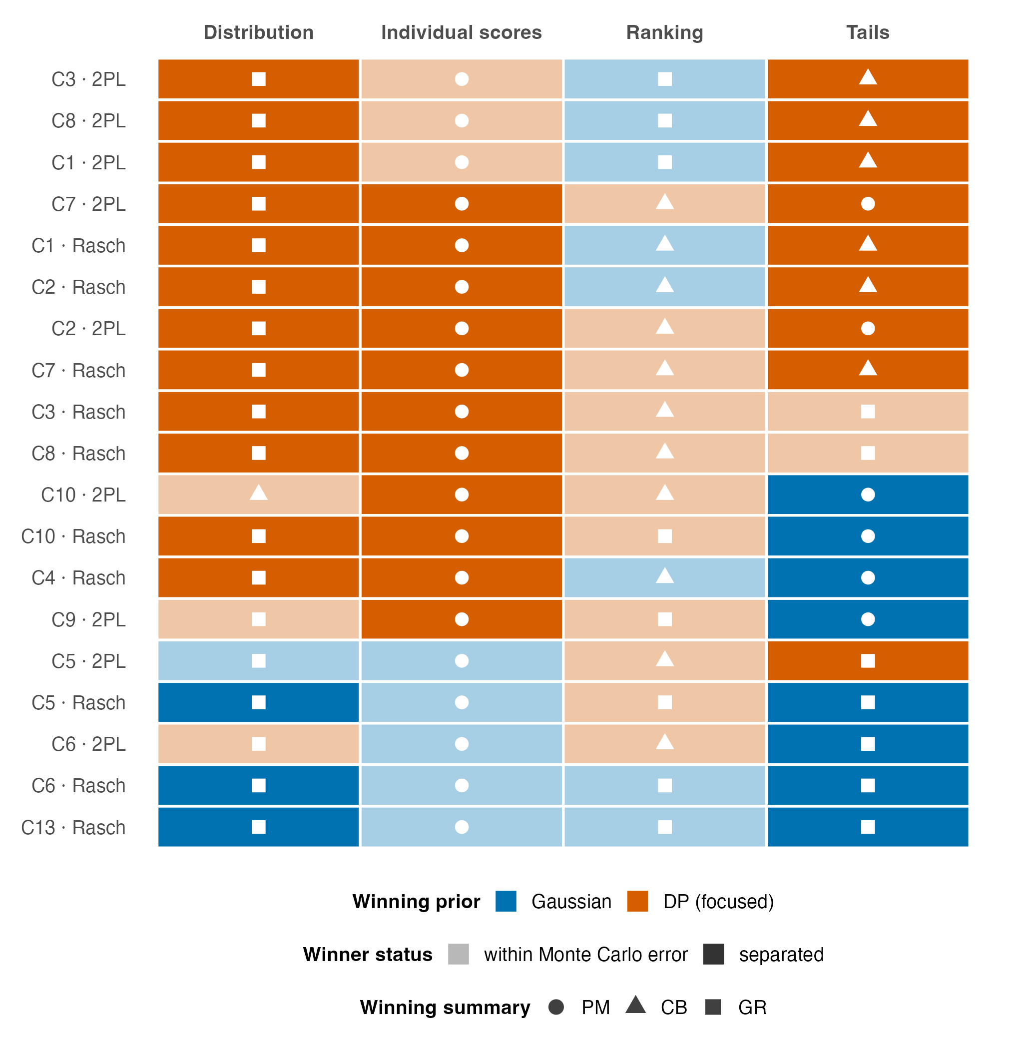
A GR combination wins the distribution goal in 18 of 19 matched cells, and a PM combination wins individual-score MSEL in 19 of 19. The summary follows the goal almost without exception; the winning prior follows the case. This is evidence about the simulated grid, read at the cells these tests occupy, and it is the only register in this book that can say which choice is better rather than merely different.

15.3 Comparator-dependent loss ratios

Against the selected six-combination winner, Gaussian + PM has a distribution-loss ratio from 1.36 to 2.54, median 2.08. This is a post-selection ratio. Directly comparing Gaussian + PM with the pre-specified Gaussian + GR comparator gives a median ratio of 1.20 overall and 1.15 on the skewed and bimodal rows. The first calculation compares the default with a selected minimum; the second isolates the change from PM to GR under the Gaussian prior.

Figure 15.2: Across the 19 matched case-cells, Gaussian + PM carries between 1.36 and 2.54 times the distribution-recovery loss of the selected six-combination winner, with a median of 2.08. Each lollipop is one matched case-cell; its length is the ratio of the default’s condition-mean KS loss to the winning combination’s, in the matched simulation cell (six-combination roster; the winner is GR under one of the priors in almost every row). The ratio is post-selection and therefore descriptive: the winner is chosen in the same cell in which it is scored. Against the pre-specified Gaussian + GR comparator, the median default-to-comparator ratio is 1.20 overall and 1.15 on the non-normal rows. The Gaussian + GR-to-winner ratio is a different estimand and is not substituted for that comparison. Shape classes are the standardized ones; the reliability side of each match is a nearest-tier approximation and every row carries its gap.

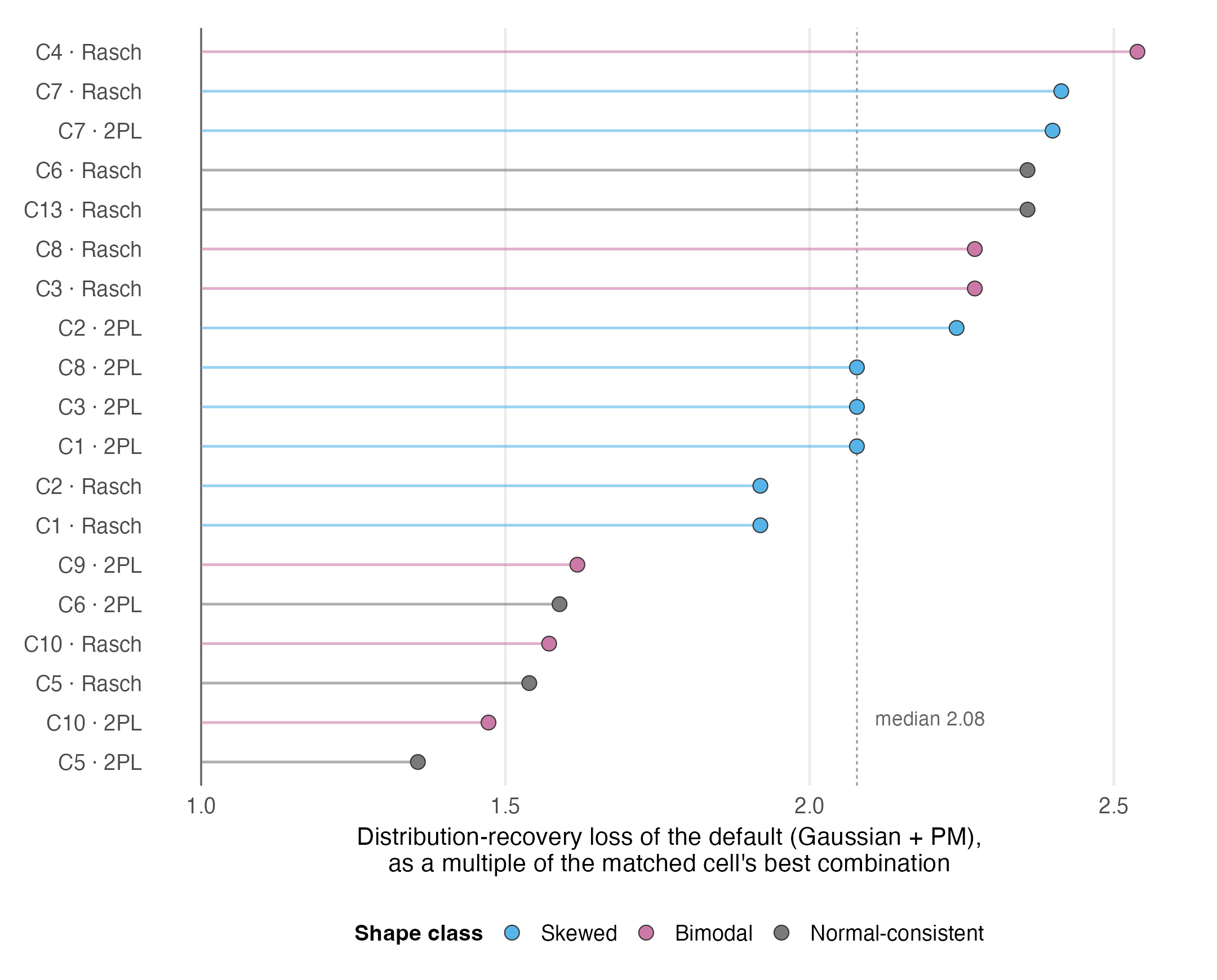
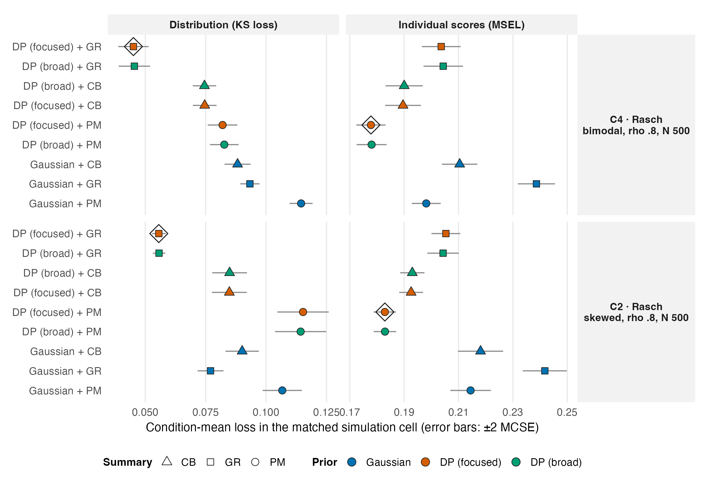
The prior and summary levers also depend on the estimand. In the 14 in-support non-normal rows, the summary-only swap beats the prior-only swap in only 3 rows. Their case-weighted geometric loss factors are 0.841 for summary-only and 0.811 for prior-only. By contrast, the simulation-wide full 3\times3 factorial decomposition assigns 82% to summary and 14% to prior. These are different estimands and are not presented as competing estimates of one quantity.

Figure 15.3 shows two full menus to make that dependence visible.

Figure 15.3: Two full menus for matched case-cells that sit at the same reliability tier and sample size and differ only in shape class. For C4–Rasch (bimodal) and C2–Rasch (skewed), all nine prior + summary combinations are represented by their condition-mean loss in the case’s matched simulation cell (rows of each panel; horizontal bars are ±2 Monte Carlo standard errors; the open diamond marks the six-combination winner). Combinations whose bars overlap are not separated by this evidence. Both case-cells carry a standardized shape class and a reliability inside the grid’s support, so both are recommendation-eligible; the reliability side of each match is still a nearest-tier approximation carrying a gap, and the plotted losses are simulation quantities rather than case-study measurements. Losses come directly from sim-v3’s condition-mean store.

15.4 What this chapter establishes, and what it does not

For every eligible non-normal case-cell, the simulation’s verdict in the matching cell favors the flexible prior for distributional reporting, by enough to matter and with the GR summary doing the larger share of the work; for every matched cell of any shape, PM remains the summary for individual scores; and the default combination, judged where these cases live, roughly doubles distributional loss relative to the attainable.

Four limits travel with those statements. The join is unpreregistered and was assembled after both source volumes’ results, so it is exploratory in status even though its inputs are frozen. The reliability match is an approximation carrying a tier gap of up to 0.049. The ordering of the two levers depends on the estimand, as the comparator analysis above shows, so no universal larger-lever claim is made here. And nothing in this chapter is validated by the cases: a case study without truth cannot confirm a simulation, and the two-register discipline of Chapter 3 is what licenses the chapter at all. Its scope is dichotomous, unidimensional data, N from 50 to 500, the three simulated shapes, a joint test-length and c^* reliability ladder, and the studied item-bank template and estimator family.