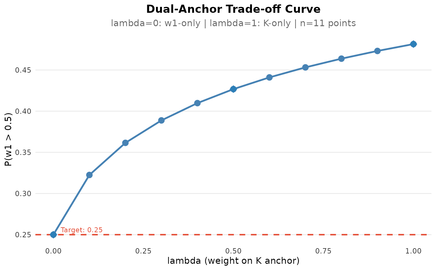
Plot Trade-off Curve — plot_tradeoff_curve • DPprior

Visualizes the Pareto trade-off between K_J fit and weight constraint across different lambda values.

Usage

plot_tradeoff_curve(
  tradeoff_data,
  metric = c("w1_prob_gt_50", "E_w1", "K_loss", "var_K"),
  target_value = NULL,
  engine = c("ggplot2", "base"),
  base_size = 11,
  title = NULL,
  show = TRUE
)

Arguments

tradeoff_data: Data frame from compute_tradeoff_curve().
metric: Which metric to plot on y-axis: "w1_prob_gt_50" (default), "E_w1", "K_loss", or "var_K".
target_value: Optional target value to mark with horizontal line.
engine: "ggplot2" (default) or "base".
base_size: Base font size.
title: Optional title.
show: If TRUE, print the plot.

Value

A ggplot object or invisible(NULL).

Examples

curve <- compute_tradeoff_curve(
  J = 50,
  K_target = list(mu_K = 5, var_K = 8),
  w1_target = list(prob = list(threshold = 0.5, value = 0.25)),
  lambda_seq = seq(0, 1, by = 0.1)
)
plot_tradeoff_curve(curve, target_value = 0.25)