Weight Distributions: w₁, ρ, and the Dual-Anchor Framework

JoonHo Lee

2026-01-01

Overview

This vignette provides a rigorous treatment of the stick-breaking weight distributions in Dirichlet Process (DP) models and their role in the dual-anchor elicitation framework. It is intended for statisticians and methodological researchers who wish to understand:

1. The distributional properties of the first stick-breaking weight $w_1$
2. The co-clustering probability $\rho = \sum_h w_h^2$ and its interpretation
3. The $I_c$ functional for computing closed-form moments under Gamma hyperpriors
4. The mathematical foundation of dual-anchor optimization

Throughout, we carefully distinguish between established results from the Bayesian nonparametrics literature and novel contributions of this work (the DPprior package and associated research notes).

Attribution Summary

Result	Attribution
Stick-breaking construction	Sethuraman (1994)
GEM distribution / size-biased ordering	Kingman (1975), Pitman (1996), Arratia et al. (2003)
$\mathbb{E}[\rho \mid \alpha] = 1/(1+\alpha)$	Kingman (1975), Pitman (1996)
Closed-form $w_1$ distribution under Gamma prior	Vicentini & Jermyn (2025)
Dual-anchor framework and $I_c$ functional formulas	This work (DPprior package)

1. Stick-Breaking Weights: Review and Interpretation

1.1 The GEM($\alpha$) Construction

Under Sethuraman’s (1994) stick-breaking representation of the DP, a random probability measure $G \sim \text{DP}(\alpha, G_0)$ can be written as: $$G = \sum_{h=1}^{\infty} w_h \, \delta_{\theta_h},$$ where $\{\theta_h\}_{h=1}^{\infty} \stackrel{iid}{\sim} G_0$ are the atom locations and $\{w_h\}_{h=1}^{\infty}$ are the stick-breaking weights constructed as: $$v_h \stackrel{iid}{\sim} \text{Beta}(1, \alpha), \quad w_1 = v_1, \quad w_h = v_h \prod_{\ell < h}(1 - v_\ell) \quad (h \geq 2).$$

The sequence $(w_1, w_2, \ldots)$ follows the GEM($\alpha$) distribution (Griffiths-Engen-McCloskey), which represents a size-biased random permutation of the Poisson-Dirichlet distribution (Pitman, 1996).

1.2 Critical Interpretability Caveat

The GEM order is size-biased, NOT decreasing.

This distinction is essential for applied elicitation. Specifically:

• $(w_1, w_2, \ldots) \neq (w_{(1)}, w_{(2)}, \ldots)$ where the latter denotes the ranked (decreasing) weights
• $w_1$ is not “the largest cluster proportion”
• A faithful interpretation: $w_1$ is the asymptotic proportion of the cluster containing a randomly selected unit (equivalently, a size-biased pick from the Poisson-Dirichlet distribution)

Despite this caveat, $w_1$ remains a meaningful diagnostic for “dominance risk.” If $P(w_1 > 0.5)$ is high, then a randomly selected unit is likely to belong to a cluster that contains more than half of the population.

# Demonstrate the stick-breaking construction
n_atoms <- 15
alpha_values <- c(0.5, 1, 2, 5)

set.seed(123)
sb_data <- do.call(rbind, lapply(alpha_values, function(a) {
  v <- rbeta(n_atoms, 1, a)
  w <- numeric(n_atoms)
  w[1] <- v[1]
  for (h in 2:n_atoms) {
    w[h] <- v[h] * prod(1 - v[1:(h-1)])
  }
  data.frame(
    atom = 1:n_atoms,
    weight = w,
    alpha = paste0("α = ", a)
  )
}))

sb_data$alpha <- factor(sb_data$alpha, levels = paste0("α = ", alpha_values))

ggplot(sb_data, aes(x = factor(atom), y = weight, fill = alpha)) +
  geom_bar(stat = "identity") +
  facet_wrap(~alpha, nrow = 1) +
  scale_fill_manual(values = palette_main) +
  labs(
    x = "Atom Index (h)", 
    y = expression(w[h]),
    title = "Stick-Breaking Weights in GEM Order",
    subtitle = "Single realization per α; NOT ranked by size"
  ) +
  theme_minimal() +
  theme(legend.position = "none")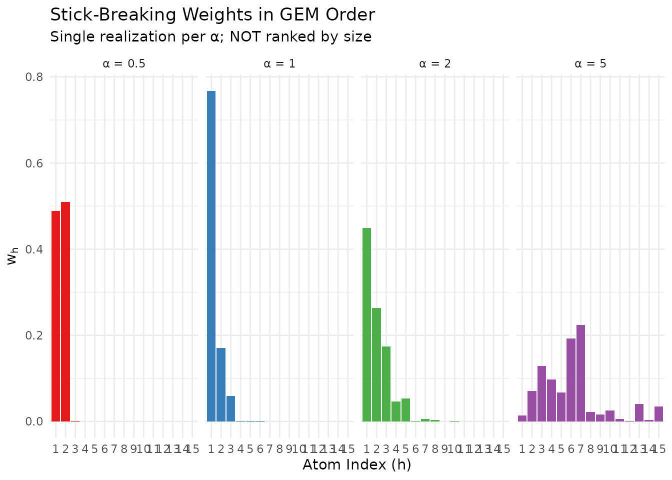

Stick-breaking weights for different α values. Smaller α concentrates mass on early atoms.

2. Distribution of $w_1$

2.1 Conditional Distribution

The first stick-breaking weight has a particularly simple conditional distribution, following directly from the construction.

Proposition 1 (Conditional distribution of $w_1$). For $\alpha > 0$: $$w_1 \mid \alpha \sim \text{Beta}(1, \alpha).$$

Consequently:

• $\mathbb{E}[w_1 \mid \alpha] = \frac{1}{1 + \alpha}$
• $\text{Var}(w_1 \mid \alpha) = \frac{\alpha}{(1+\alpha)^2(2+\alpha)}$
• $P(w_1 \leq x \mid \alpha) = 1 - (1-x)^{\alpha}$ for $x \in [0, 1]$

Attribution: This follows immediately from the stick-breaking construction (Sethuraman, 1994).

x_grid <- seq(0.001, 0.999, length.out = 200)
alpha_grid <- c(0.5, 1, 2, 5, 10)

cond_df <- do.call(rbind, lapply(alpha_grid, function(a) {
  data.frame(
    x = x_grid,
    density = dbeta(x_grid, 1, a),
    alpha = paste0("α = ", a)
  )
}))
cond_df$alpha <- factor(cond_df$alpha, levels = paste0("α = ", alpha_grid))

ggplot(cond_df, aes(x = x, y = density, color = alpha)) +
  geom_line(linewidth = 0.9) +
  scale_color_viridis_d(option = "plasma", end = 0.85) +
  labs(
    x = expression(w[1]),
    y = "Density",
    title = expression("Conditional Density: " * w[1] * " | " * alpha * " ~ Beta(1, " * alpha * ")"),
    color = NULL
  ) +
  coord_cartesian(ylim = c(0, 6)) +
  theme_minimal() +
  theme(legend.position = "right")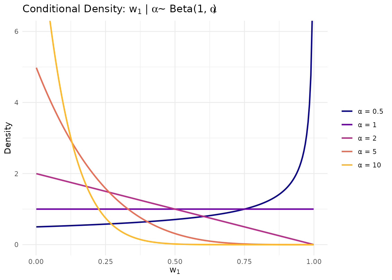

Conditional density of w₁|α for different concentration parameter values.

2.2 Marginal Distribution Under Gamma Hyperprior

When $\alpha \sim \text{Gamma}(a, b)$ with shape $a > 0$ and rate $b > 0$, the unconditional distribution of $w_1$ admits fully closed-form expressions.

Theorem 1 (Unconditional distribution of $w_1$; Vicentini & Jermyn, 2025, Appendix A). Let $\alpha \sim \text{Gamma}(a, b)$. Then:

Density: $$p(w_1 \mid a, b) = \frac{a \, b^a}{(1 - w_1)[b - \log(1-w_1)]^{a+1}}, \quad w_1 \in (0, 1).$$

CDF: $$F_{w_1}(x \mid a, b) = P(w_1 \leq x \mid a, b) = 1 - \left(\frac{b}{b - \log(1-x)}\right)^a.$$

Survival function (dominance risk): $$P(w_1 > t \mid a, b) = \left(\frac{b}{b - \log(1-t)}\right)^a.$$

Quantile function: $$Q_{w_1}(u \mid a, b) = 1 - \exp\left(b\left[1 - (1-u)^{-1/a}\right]\right).$$

Proof sketch. Integrate out $\alpha$ from the conditional distribution: $$p(w_1 \mid a, b) = \int_0^\infty \alpha (1-w_1)^{\alpha-1} \cdot \frac{b^a}{\Gamma(a)} \alpha^{a-1} e^{-b\alpha} \, d\alpha.$$ The integral evaluates to a Gamma function, and the CDF follows by direct integration with substitution $u = b - \log(1-w)$. $\square$

Computational significance. These closed-form expressions enable $O(1)$ computation of quantiles and tail probabilities—no Monte Carlo sampling is required.

# Demonstrate the closed-form w1 distribution functions
a <- 1.6
b <- 1.22  # The Lee et al. DP-inform prior

cat("w₁ distribution under Gamma(a=1.6, b=1.22) hyperprior:\n")
#> w₁ distribution under Gamma(a=1.6, b=1.22) hyperprior:
cat(sprintf("  Mean:     %.4f\n", mean_w1(a, b)))
#>   Mean:     0.5084
cat(sprintf("  Variance: %.4f\n", var_w1(a, b)))
#>   Variance: 0.1052
cat(sprintf("  Median:   %.4f\n", quantile_w1(0.5, a, b)))
#>   Median:   0.4839
cat(sprintf("  90th %%:   %.4f\n", quantile_w1(0.9, a, b)))
#>   90th %:   0.9803

cat("\nDominance risk (tail probabilities):\n")
#> 
#> Dominance risk (tail probabilities):
for (t in c(0.3, 0.5, 0.7, 0.9)) {
  cat(sprintf("  P(w₁ > %.1f) = %.4f\n", t, prob_w1_exceeds(t, a, b)))
}
#>   P(w₁ > 0.3) = 0.6634
#>   P(w₁ > 0.5) = 0.4868
#>   P(w₁ > 0.7) = 0.3334
#>   P(w₁ > 0.9) = 0.1833

2.3 Visualization of the Marginal Distribution

# Visualize the marginal w1 distribution
x_grid <- seq(0.01, 0.99, length.out = 200)
a <- 1.6
b <- 1.22

# Compute density manually using the closed-form formula
# p(w1 | a, b) = a * b^a / ((1-w1) * (b - log(1-w1))^(a+1))
density_w1_manual <- function(x, a, b) {
  denom <- (1 - x) * (b - log(1 - x))^(a + 1)
  a * b^a / denom
}

w1_df <- data.frame(
  x = x_grid,
  density = density_w1_manual(x_grid, a, b),
  cdf = cdf_w1(x_grid, a, b),
  survival = prob_w1_exceeds(x_grid, a, b)
)

p1 <- ggplot(w1_df, aes(x = x, y = density)) +
  geom_line(color = "#E41A1C", linewidth = 1) +
  geom_vline(xintercept = quantile_w1(0.5, a, b), linetype = "dashed", 
             color = "#377EB8", alpha = 0.7) +
  annotate("text", x = quantile_w1(0.5, a, b) + 0.05, y = max(w1_df$density) * 0.9,
           label = "Median", color = "#377EB8", hjust = 0) +
  labs(x = expression(w[1]), y = "Density",
       title = expression("Marginal Density of " * w[1] * " | Gamma(1.6, 1.22)")) +
  theme_minimal()

p2 <- ggplot(w1_df, aes(x = x)) +
  geom_line(aes(y = cdf), color = "#377EB8", linewidth = 1) +
  geom_line(aes(y = survival), color = "#E41A1C", linewidth = 1, linetype = "dashed") +
  geom_hline(yintercept = 0.5, linetype = "dotted", color = "gray50") +
  annotate("text", x = 0.9, y = 0.85, label = "CDF", color = "#377EB8") +
  annotate("text", x = 0.9, y = 0.35, label = "P(w1 > x)", color = "#E41A1C") +
  labs(x = expression(w[1]), y = "Probability",
       title = "CDF and Survival Function") +
  theme_minimal()

gridExtra::grid.arrange(p1, p2, ncol = 2)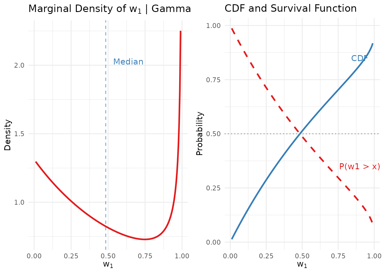

Marginal density and CDF of w₁ under the Gamma(1.6, 1.22) hyperprior.

3. The Co-Clustering Probability $\rho$

3.1 Definition and Interpretation

The co-clustering probability provides an alternative, often more intuitive, anchor for weight-based elicitation.

Definition 1 (Co-clustering probability / Simpson index). $$\rho := \sum_{h=1}^{\infty} w_h^2 \in (0, 1).$$

Interpretation. Conditional on the random measure $G$, if $Z_1, Z_2$ are i.i.d. cluster labels with $P(Z = k \mid G) = w_k$, then: $$P(Z_1 = Z_2 \mid G) = \sum_{k \geq 1} w_k^2 = \rho.$$

Thus $\rho$ is the probability that two randomly chosen units belong to the same latent cluster. This quantity translates directly to applied elicitation:

“Before seeing data, what is the probability that two randomly selected sites from your study belong to the same effect group?”

3.2 Conditional Moments of $\rho$

Proposition 2 (Conditional expectation of $\rho$; Kingman, 1975; Pitman, 1996). $$\mathbb{E}[\rho \mid \alpha] = \frac{1}{1 + \alpha}.$$

Proof. Using the stick-breaking construction: $$\mathbb{E}[w_k^2 \mid \alpha] = \mathbb{E}[v_k^2] \cdot \prod_{\ell < k} \mathbb{E}[(1-v_\ell)^2].$$

For $v \sim \text{Beta}(1, \alpha)$: $$\mathbb{E}[v^2] = \frac{2}{(1+\alpha)(2+\alpha)}, \quad \mathbb{E}[(1-v)^2] = \frac{\alpha}{2+\alpha}.$$

Summing the geometric series: $$\mathbb{E}[\rho \mid \alpha] = \sum_{k=1}^\infty \frac{2}{(1+\alpha)(2+\alpha)} \left(\frac{\alpha}{2+\alpha}\right)^{k-1} = \frac{1}{1+\alpha}.$$$\square$

Corollary 1 (Key identity). The conditional expectations of $w_1$ and $\rho$ are equal: $$\mathbb{E}[w_1 \mid \alpha] = \mathbb{E}[\rho \mid \alpha] = \frac{1}{1+\alpha}.$$

This identity is not coincidental—both quantities measure the “concentration” of the random measure $G$.

Proposition 3 (Conditional variance of $\rho$). $$\mathbb{E}[\rho^2 \mid \alpha] = \frac{\alpha + 6}{(\alpha+1)(\alpha+2)(\alpha+3)},$$$$\text{Var}(\rho \mid \alpha) = \frac{2\alpha}{(\alpha+1)^2(\alpha+2)(\alpha+3)}.$$

Proof. Using the distributional recursion $\rho \stackrel{d}{=} v^2 + (1-v)^2 \rho'$ where $v \sim \text{Beta}(1, \alpha)$ and $\rho'$ is an independent copy of $\rho$. Squaring and taking expectations yields the result. See Appendix A of the associated research notes for the full derivation. $\square$

alpha_grid <- seq(0.1, 20, length.out = 200)

rho_cond_df <- data.frame(
  alpha = alpha_grid,
  mean = mean_rho_given_alpha(alpha_grid),
  var = var_rho_given_alpha(alpha_grid),
  sd = sqrt(var_rho_given_alpha(alpha_grid))
)

p1 <- ggplot(rho_cond_df, aes(x = alpha, y = mean)) +
  geom_line(color = "#E41A1C", linewidth = 1) +
  geom_ribbon(aes(ymin = pmax(0, mean - 2*sd), ymax = pmin(1, mean + 2*sd)), 
              alpha = 0.2, fill = "#E41A1C") +
  labs(x = expression(alpha), y = expression(rho),
       title = expression(E*"["*rho*" | "*alpha*"]" * " ± 2 SD")) +
  coord_cartesian(ylim = c(0, 1)) +
  theme_minimal()

p2 <- ggplot(rho_cond_df, aes(x = alpha, y = var)) +
  geom_line(color = "#377EB8", linewidth = 1) +
  labs(x = expression(alpha), y = "Variance",
       title = expression("Var("*rho*" | "*alpha*")")) +
  theme_minimal()

gridExtra::grid.arrange(p1, p2, ncol = 2)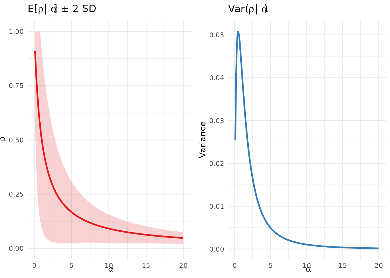

Conditional mean and variance of ρ as functions of α.

4. The $I_c$ Functional: Closed-Form Moments

4.1 Definition and Analytical Expression

Computing unconditional moments of $w_1$ and $\rho$ under a Gamma hyperprior requires evaluating expectations of the form $\mathbb{E}[1/(\alpha + c)]$.

Definition 2 (The $I_c$ functional). $$I_c(a, b) := \mathbb{E}\left[\frac{1}{\alpha + c}\right], \quad \text{where } \alpha \sim \text{Gamma}(a, b) \text{ and } c > 0.$$

Lemma 1 (Closed-form expression for $I_c$; this work). $$I_c(a, b) = b^a \, c^{a-1} \, e^{bc} \, \Gamma(1-a, bc),$$ where $\Gamma(s, x) = \int_x^\infty t^{s-1} e^{-t} \, dt$ is the upper incomplete gamma function.

Proof. We have: $$I_c(a, b) = \frac{b^a}{\Gamma(a)} \int_0^\infty \frac{\alpha^{a-1} e^{-b\alpha}}{\alpha + c} \, d\alpha.$$

Using the integral identity: $$\int_0^\infty \frac{x^{a-1} e^{-bx}}{x + c} \, dx = c^{a-1} e^{bc} \Gamma(a) \Gamma(1-a, bc),$$ and multiplying by $b^a / \Gamma(a)$, we obtain the result. $\square$

Remark 1 (Numerical evaluation). For $a > 1$, the upper incomplete gamma function $\Gamma(1-a, bc)$ is defined via analytic continuation. Standard numerical libraries handle this automatically (e.g., pgamma in R with appropriate transformations, or scipy.special.gammaincc in Python). For practical purposes in the DPprior package, we use Gauss-Laguerre quadrature which avoids these analytic continuation subtleties.

4.2 Key Identities

Theorem 2 (Unconditional moments via $I_c$; this work).

Let $\alpha \sim \text{Gamma}(a, b)$. Then:

Mean of $w_1$: $$\mathbb{E}[w_1 \mid a, b] = \mathbb{E}\left[\frac{1}{1+\alpha}\right] = I_1(a, b).$$

Mean of $\rho$ (co-clustering probability): $$\mathbb{E}[\rho \mid a, b] = \mathbb{E}\left[\frac{1}{1+\alpha}\right] = I_1(a, b).$$

Corollary 2 (Moment identity). The unconditional means are equal: $$\mathbb{E}[w_1 \mid a, b] = \mathbb{E}[\rho \mid a, b] = I_1(a, b).$$

This identity has important implications for elicitation: if a practitioner specifies only a target for the mean of $w_1$ or $\rho$, the two anchors are informationally equivalent. To make $\rho$ add genuine extra constraint, one must elicit uncertainty (e.g., an interval) and match the variance.

# Verify the key identity: E[w1] = E[rho]
test_cases <- list(
  c(a = 1.0, b = 1.0),
  c(a = 1.6, b = 1.22),
  c(a = 2.0, b = 0.5),
  c(a = 0.5, b = 2.0)
)

cat("Verification: E[w₁] = E[ρ] identity\n")
#> Verification: E[w₁] = E[ρ] identity
cat(sprintf("%10s %10s %12s %12s %12s\n", "a", "b", "E[w₁]", "E[ρ]", "Difference"))
#>          a          b      E[w₁]        E[ρ]   Difference
cat(strrep("-", 60), "\n")
#> ------------------------------------------------------------

for (params in test_cases) {
  a <- params["a"]
  b <- params["b"]
  E_w1 <- mean_w1(a, b)
  E_rho <- mean_rho(a, b)
  diff <- abs(E_w1 - E_rho)
  cat(sprintf("%10.2f %10.2f %12.6f %12.6f %12.2e\n", a, b, E_w1, E_rho, diff))
}
#>       1.00       1.00     0.596347     0.596347     0.00e+00
#>       1.60       1.22     0.508368     0.508368     0.00e+00
#>       2.00       0.50     0.269272     0.269272     0.00e+00
#>       0.50       2.00     0.842738     0.842738     0.00e+00

4.3 Second Moments and Variance of $\rho$

Proposition 4 (Unconditional second moment of $\rho$; this work).

Using the partial fraction decomposition: $$\frac{\alpha + 6}{(\alpha+1)(\alpha+2)(\alpha+3)} = \frac{5}{2(\alpha+1)} - \frac{4}{\alpha+2} + \frac{3}{2(\alpha+3)},$$

we obtain: $$\mathbb{E}[\rho^2 \mid a, b] = \frac{5}{2} I_1(a, b) - 4 I_2(a, b) + \frac{3}{2} I_3(a, b).$$

Hence the unconditional variance: $$\text{Var}(\rho \mid a, b) = \mathbb{E}[\rho^2 \mid a, b] - \{\mathbb{E}[\rho \mid a, b]\}^2.$$

Key design implication. The distribution of $\rho \mid a, b$ is not closed-form, but mean and variance are closed-form (“moment-closed”). This is sufficient for moment-based calibration and diagnostics.

# Compute unconditional rho moments for the Lee et al. prior
a <- 1.6
b <- 1.22

cat("Co-clustering probability under Gamma(1.6, 1.22) hyperprior:\n")
#> Co-clustering probability under Gamma(1.6, 1.22) hyperprior:
cat(sprintf("  E[ρ]   = %.4f\n", mean_rho(a, b)))
#>   E[ρ]   = 0.5084
cat(sprintf("  Var(ρ) = %.4f\n", var_rho(a, b)))
#>   Var(ρ) = 0.0710
cat(sprintf("  SD(ρ)  = %.4f\n", sqrt(var_rho(a, b))))
#>   SD(ρ)  = 0.2664
cat(sprintf("  CV(ρ)  = %.4f\n", cv_rho(a, b)))
#>   CV(ρ)  = 0.5240

5. The Dual-Anchor Optimization Framework

5.1 Motivation: Why K-Only Calibration is Insufficient

As demonstrated by Vicentini and Jermyn (2025, Section 5), priors calibrated to match a target on the number of clusters $K_J$ can induce materially informative priors on the stick-breaking weights. They observe that “$K_n$-diffuse, DORO, quasi-degenerate and Jeffreys’ priors… are markedly different from the behaviour of SSI” (p. 18).

The mechanism is structural: $K_J$ and the weight distribution are controlled by different functionals of $\alpha$. For fixed $J$: $$\mathbb{E}[K_J \mid \alpha] \approx 1 + \alpha \log J \quad \text{(Antoniak, 1974)},$$ while: $$\mathbb{E}[w_1 \mid \alpha] = \frac{1}{1 + \alpha}.$$

Matching the location of $K_J$ pins down $\alpha$ around $\alpha \approx (\mathbb{E}[K_J] - 1)/\log J$, but this implied $\alpha$ can correspond to high dominance risk in $w_1$.

# Demonstrate the unintended prior problem
J <- 50
mu_K_target <- 5

# Fit using K-only calibration
fit_K <- DPprior_fit(J = J, mu_K = mu_K_target, confidence = "medium")
#> Warning: HIGH DOMINANCE RISK: P(w1 > 0.5) = 49.7% exceeds 40%.
#>   This may indicate unintended prior behavior (RN-07).
#>   Consider using DPprior_dual() for weight-constrained elicitation.
#>   See ?DPprior_diagnostics for interpretation.

# What does this imply for weights?
cat("K-only calibration (J=50, μ_K=5):\n")
#> K-only calibration (J=50, μ_K=5):
cat(sprintf("  Gamma hyperprior: a = %.3f, b = %.3f\n", fit_K$a, fit_K$b))
#>   Gamma hyperprior: a = 1.408, b = 1.077
cat(sprintf("  Achieved E[K] = %.2f\n", 
            exact_K_moments(J, fit_K$a, fit_K$b)$mean))
#>   Achieved E[K] = 5.00
cat("\nImplied weight behavior:\n")
#> 
#> Implied weight behavior:
cat(sprintf("  E[w₁] = %.3f\n", mean_w1(fit_K$a, fit_K$b)))
#>   E[w₁] = 0.518
cat(sprintf("  P(w₁ > 0.5) = %.3f\n", prob_w1_exceeds(0.5, fit_K$a, fit_K$b)))
#>   P(w₁ > 0.5) = 0.497
cat(sprintf("  P(w₁ > 0.9) = %.3f\n", prob_w1_exceeds(0.9, fit_K$a, fit_K$b)))
#>   P(w₁ > 0.9) = 0.200

# Visualize the implied w1 distribution
x_grid <- seq(0.01, 0.99, length.out = 200)

implied_df <- data.frame(
  x = x_grid,
  density = density_w1_manual(x_grid, fit_K$a, fit_K$b),
  type = "K-only calibration"
)

ggplot(implied_df, aes(x = x, y = density)) +
  geom_line(color = "#377EB8", linewidth = 1.2) +
  geom_vline(xintercept = 0.5, linetype = "dashed", color = "#E41A1C", alpha = 0.7) +
  annotate("text", x = 0.52, y = max(implied_df$density) * 0.8, 
           label = "50% threshold", color = "#E41A1C", hjust = 0) +
  labs(
    x = expression(w[1]),
    y = "Density",
    title = expression("Implied Distribution of " * w[1] * " Under K-Only Calibration"),
    subtitle = sprintf("J = %d, target E[K] = %d; P(w₁ > 0.5) = %.2f", 
                       J, mu_K_target, prob_w1_exceeds(0.5, fit_K$a, fit_K$b))
  ) +
  theme_minimal()

The K-calibrated prior (blue) achieves the target E[K] but implies higher dominance risk than practitioners might expect.

5.2 The Dual-Anchor Objective

Definition 3 (Dual-anchor optimization; this work).

Given elicited targets $p^*(K_J)$ (or summary statistics thereof) and $p^*(T)$ where $T \in \{w_1, \rho\}$, the dual-anchor hyperparameters are: $$(a^*, b^*) = \arg\min_{a > 0, b > 0} \mathcal{L}_\lambda(a, b),$$where: $$\mathcal{L}_\lambda(a, b) = \lambda \cdot D\{p^*(K_J) \| p_{a,b}(K_J)\} + (1 - \lambda) \cdot D\{p^*(T) \| p_{a,b}(T)\},$$and $\lambda \in [0, 1]$ controls the trade-off between the two anchors.

Boundary cases:

$\lambda$	Behavior
$\lambda = 1$	K-only calibration (RN-01 through RN-05)
$\lambda = 0$	Weight-only calibration (SSI-style)
$0 < \lambda < 1$	Compromise between both anchors

5.3 Implementation Variants

The dual-anchor objective can be implemented using different loss functions:

Moment-based loss (recommended for stability): $$\mathcal{L}(a, b) = \lambda \left[(\mathbb{E}[K_J] - \mu_K^*)^2 + \omega_K (\text{Var}(K_J) - \sigma_K^{2*})^2\right] + (1 - \lambda) \left[(\mathbb{E}[T] - \mu_T^*)^2 + \omega_T (\text{Var}(T) - \sigma_T^{2*})^2\right],$$ where $\omega_K, \omega_T \geq 0$ are tuning weights.

Quantile-based loss for $w_1$: For $T = w_1$, one can directly target specific quantiles using the closed-form $Q_{w_1}$: $$\mathcal{L}(a, b) = \lambda \cdot L_K(a, b) + (1 - \lambda) \sum_{i} \left[Q_{w_1}(u_i \mid a, b) - q_i^*\right]^2,$$ where $(u_i, q_i^*)$ are elicited quantile pairs.

Probability constraint for $w_1$: Target a specific dominance risk: $$\mathcal{L}(a, b) = \lambda \cdot L_K(a, b) + (1 - \lambda) \left[P(w_1 > t \mid a, b) - p_t^*\right]^2.$$

# Demonstrate dual-anchor calibration
fit_dual <- DPprior_dual(
  fit = fit_K,
  w1_target = list(prob = list(threshold = 0.5, value = 0.25)),
  lambda = 0.7,
  loss_type = "adaptive",
  verbose = FALSE
)

cat("Dual-anchor calibration (target: P(w₁ > 0.5) = 0.25):\n")
#> Dual-anchor calibration (target: P(w₁ > 0.5) = 0.25):
cat(sprintf("  Gamma hyperprior: a = %.3f, b = %.3f\n", fit_dual$a, fit_dual$b))
#>   Gamma hyperprior: a = 3.078, b = 1.669
cat(sprintf("  Achieved E[K] = %.2f (target: %.1f)\n", 
            exact_K_moments(J, fit_dual$a, fit_dual$b)$mean, mu_K_target))
#>   Achieved E[K] = 6.43 (target: 5.0)
cat(sprintf("  P(w₁ > 0.5) = %.3f (target: 0.25)\n", 
            prob_w1_exceeds(0.5, fit_dual$a, fit_dual$b)))
#>   P(w₁ > 0.5) = 0.343 (target: 0.25)

5.4 The Trade-off Curve

# Compute trade-off curve
lambda_grid <- c(1.0, 0.9, 0.8, 0.7, 0.6, 0.5, 0.4, 0.3)
w1_target <- list(prob = list(threshold = 0.5, value = 0.2))

tradeoff_results <- lapply(lambda_grid, function(lam) {
  if (lam == 1.0) {
    fit <- fit_K
    fit$dual_anchor <- list(lambda = 1.0)
  } else {
    fit <- DPprior_dual(fit_K, w1_target, lambda = lam, 
                        loss_type = "adaptive", verbose = FALSE)
  }
  
  list(
    lambda = lam,
    a = fit$a,
    b = fit$b,
    E_K = exact_K_moments(J, fit$a, fit$b)$mean,
    P_w1_gt_50 = prob_w1_exceeds(0.5, fit$a, fit$b),
    E_w1 = mean_w1(fit$a, fit$b)
  )
})

tradeoff_df <- data.frame(
  lambda = sapply(tradeoff_results, `[[`, "lambda"),
  E_K = sapply(tradeoff_results, `[[`, "E_K"),
  P_w1 = sapply(tradeoff_results, `[[`, "P_w1_gt_50"),
  E_w1 = sapply(tradeoff_results, `[[`, "E_w1")
)

ggplot(tradeoff_df, aes(x = E_K, y = P_w1)) +
  geom_path(color = "gray50", linewidth = 0.8) +
  geom_point(aes(color = factor(lambda)), size = 4) +
  geom_hline(yintercept = 0.2, linetype = "dashed", color = "#E41A1C", alpha = 0.7) +
  geom_vline(xintercept = 5, linetype = "dashed", color = "#377EB8", alpha = 0.7) +
  annotate("text", x = 4.5, y = 0.22, label = "w1 target", 
           hjust = 1, color = "#E41A1C") +
  annotate("text", x = 5.1, y = 0.45, label = "K target", hjust = 0, color = "#377EB8") +
  scale_color_viridis_d(option = "viridis", begin = 0.2, end = 0.8) +
  labs(
    x = expression(E*"["*K[J]*"]"),
    y = expression(P(w[1] > 0.5)),
    title = "Dual-Anchor Trade-off Curve",
    subtitle = "Varying λ from 1.0 (K-only) to 0.3 (weight-priority)",
    color = "λ"
  ) +
  theme_minimal() +
  theme(legend.position = "right")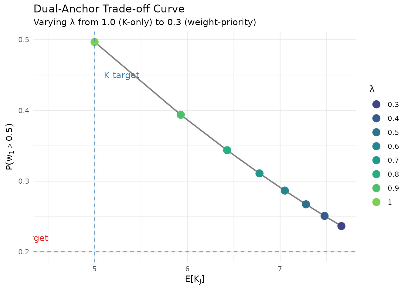

Trade-off between K-fit and weight control as λ varies from 1 (K-only) to 0.3 (weight-priority).

6. Relationship Between $w_1$ and $\rho$

6.1 When Are They Equivalent?

As established above, $\mathbb{E}[w_1 \mid \alpha] = \mathbb{E}[\rho \mid \alpha]$. This extends to the unconditional case: $\mathbb{E}[w_1 \mid a, b] = \mathbb{E}[\rho \mid a, b]$.

Consequence: If the practitioner elicits only a mean constraint (e.g., “co-clustering probability should be about 0.3”), using $w_1$ or $\rho$ as the second anchor yields identical calibration constraints.

6.2 When Are They Different?

The variances differ: $$\text{Var}(w_1 \mid \alpha) = \frac{\alpha}{(1+\alpha)^2(2+\alpha)} \neq \text{Var}(\rho \mid \alpha) = \frac{2\alpha}{(\alpha+1)^2(\alpha+2)(\alpha+3)}.$$

alpha_grid <- seq(0.1, 20, length.out = 200)

var_comparison <- data.frame(
  alpha = rep(alpha_grid, 2),
  variance = c(
    alpha_grid / ((1 + alpha_grid)^2 * (2 + alpha_grid)),  # Var(w1|alpha)
    var_rho_given_alpha(alpha_grid)                          # Var(rho|alpha)
  ),
  quantity = rep(c("Var(w₁ | α)", "Var(ρ | α)"), each = length(alpha_grid))
)

ggplot(var_comparison, aes(x = alpha, y = variance, color = quantity)) +
  geom_line(linewidth = 1) +
  scale_color_manual(values = c("#E41A1C", "#377EB8")) +
  labs(
    x = expression(alpha),
    y = "Conditional Variance",
    title = expression("Conditional Variance Comparison: " * w[1] * " vs " * rho),
    color = NULL
  ) +
  theme_minimal() +
  theme(legend.position = "bottom")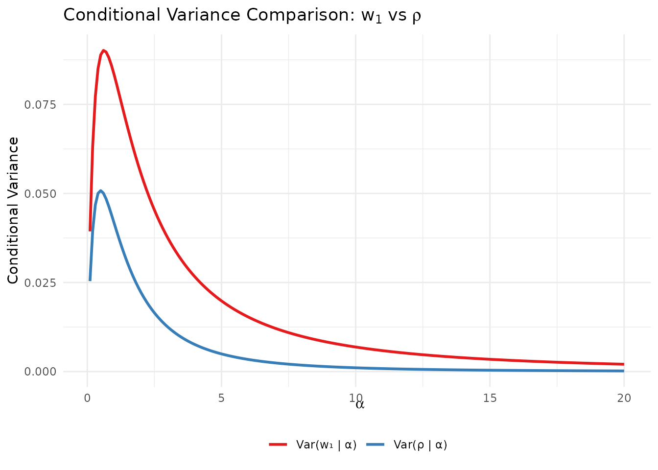

Comparison of conditional variances: Var(w₁|α) vs Var(ρ|α).

6.3 Practical Guidance: Choosing Between $w_1$ and $\rho$

Criterion	$w_1$	$\rho$
Distribution tractability	Fully closed-form (CDF, quantiles)	Moment-closed only
Elicitation intuitiveness	Moderate	High (“probability two share a cluster”)
Tail constraints	Direct via $P(w_1 > t)$	Requires simulation
Variance matching	Possible but complex	Straightforward

Recommendation: Use $w_1$ for quantile/probability constraints; use $\rho$ when the co-clustering interpretation resonates with domain experts.

7. Computational Details

7.1 Key Functions in the DPprior Package

The package provides efficient implementations for all weight-related computations:

Function	Description
mean_w1(a, b)	$\mathbb{E}[w_1 \mid a, b]$ via Gauss-Laguerre quadrature
var_w1(a, b)	$\text{Var}(w_1 \mid a, b)$ via quadrature
cdf_w1(x, a, b)	Closed-form CDF $P(w_1 \leq x)$
quantile_w1(u, a, b)	Closed-form quantile function
prob_w1_exceeds(t, a, b)	Closed-form $P(w_1 > t)$
mean_rho(a, b)	$\mathbb{E}[\rho \mid a, b]$ via quadrature
var_rho(a, b)	$\text{Var}(\rho \mid a, b)$ via quadrature
mean_rho_given_alpha(alpha)	Conditional mean $1/(1+\alpha)$
var_rho_given_alpha(alpha)	Conditional variance
DPprior_dual()	Dual-anchor calibration

7.2 Numerical Verification

# Verify implementations against Monte Carlo
a <- 1.6
b <- 1.22
n_mc <- 100000

set.seed(42)
alpha_samples <- rgamma(n_mc, shape = a, rate = b)
w1_samples <- rbeta(n_mc, 1, alpha_samples)

cat("Verification against Monte Carlo (n =", format(n_mc, big.mark = ","), "):\n\n")
#> Verification against Monte Carlo (n = 1e+05 ):

cat("w₁ moments:\n")
#> w₁ moments:
cat(sprintf("  E[w₁]: Analytic = %.4f, MC = %.4f\n", 
            mean_w1(a, b), mean(w1_samples)))
#>   E[w₁]: Analytic = 0.5084, MC = 0.5088
cat(sprintf("  Var(w₁): Analytic = %.4f, MC = %.4f\n", 
            var_w1(a, b), var(w1_samples)))
#>   Var(w₁): Analytic = 0.1052, MC = 0.1054

cat("\nw₁ tail probabilities:\n")
#> 
#> w₁ tail probabilities:
for (t in c(0.3, 0.5, 0.9)) {
  mc_prob <- mean(w1_samples > t)
  analytic_prob <- prob_w1_exceeds(t, a, b)
  cat(sprintf("  P(w₁ > %.1f): Analytic = %.4f, MC = %.4f\n", 
              t, analytic_prob, mc_prob))
}
#>   P(w₁ > 0.3): Analytic = 0.6634, MC = 0.6627
#>   P(w₁ > 0.5): Analytic = 0.4868, MC = 0.4876
#>   P(w₁ > 0.9): Analytic = 0.1833, MC = 0.1858

cat("\nρ moments (via quadrature vs MC simulation):\n")
#> 
#> ρ moments (via quadrature vs MC simulation):
rho_samples <- sapply(alpha_samples, function(alph) {
  v <- rbeta(100, 1, alph)
  w <- cumprod(c(1, 1 - v[-length(v)])) * v
  sum(w^2)
})
cat(sprintf("  E[ρ]: Analytic = %.4f, MC = %.4f\n", 
            mean_rho(a, b), mean(rho_samples)))
#>   E[ρ]: Analytic = 0.5084, MC = 0.5081

8. Summary

This vignette has provided a rigorous treatment of the weight distribution theory underlying the DPprior package:

1. Stick-breaking weights $(w_1, w_2, \ldots)$ follow the GEM($\alpha$) distribution in size-biased (not decreasing) order.

2. $w_1 \mid \alpha \sim \text{Beta}(1, \alpha)$, and under $\alpha \sim \text{Gamma}(a, b)$, the marginal distribution of $w_1$ has fully closed-form CDF, quantiles, and tail probabilities.

3. The co-clustering probability $\rho = \sum_h w_h^2$ has the same conditional mean as $w_1$: $\mathbb{E}[\rho \mid \alpha] = 1/(1+\alpha)$.

4. The $I_c$ functional enables closed-form computation of $\mathbb{E}[1/(\alpha + c)]$, which underlies the moment formulas for both $w_1$ and $\rho$.

5. K-only calibration can induce unintended weight behavior. The dual-anchor framework provides explicit control over both cluster counts and weight concentration via a trade-off parameter $\lambda$.

References

Antoniak, C. E. (1974). Mixtures of Dirichlet processes with applications to Bayesian nonparametric problems. The Annals of Statistics, 2(6), 1152-1174.

Arratia, R., Barbour, A. D., & Tavaré, S. (2003). Logarithmic Combinatorial Structures: A Probabilistic Approach. European Mathematical Society.

Connor, R. J., & Mosimann, J. E. (1969). Concepts of independence for proportions with a generalization of the Dirichlet distribution. Journal of the American Statistical Association, 64(325), 194-206.

Dorazio, R. M. (2009). On selecting a prior for the precision parameter of Dirichlet process mixture models. Journal of Statistical Planning and Inference, 139(10), 3384-3390.

Escobar, M. D., & West, M. (1995). Bayesian density estimation and inference using mixtures. Journal of the American Statistical Association, 90(430), 577-588.

Kingman, J. F. C. (1975). Random discrete distributions. Journal of the Royal Statistical Society: Series B, 37(1), 1-22.

Lee, J., Che, J., Rabe-Hesketh, S., Feller, A., & Miratrix, L. (2025). Improving the estimation of site-specific effects and their distribution in multisite trials. Journal of Educational and Behavioral Statistics, 50(5), 731-764.

Murugiah, S., & Sweeting, T. J. (2012). Selecting the precision parameter prior in Dirichlet process mixture models. Journal of Statistical Planning and Inference, 142(7), 1947-1959.

Pitman, J. (1996). Random discrete distributions invariant under size-biased permutation. Advances in Applied Probability, 28(2), 525-539.

Sethuraman, J. (1994). A constructive definition of Dirichlet priors. Statistica Sinica, 4(2), 639-650.

Vicentini, S., & Jermyn, I. H. (2025). Prior selection for the precision parameter of Dirichlet process mixture models. arXiv:2502.00864.

Zito, A., Rigon, T., & Dunson, D. B. (2024). Bayesian nonparametric modeling of latent partitions via Stirling-gamma priors. Bayesian Analysis. https://doi.org/10.1214/24-BA1463

---

Appendix: Key Formulas Reference

A.1 Conditional Distributions

Quantity	Distribution/Moment
$w_1 \mid \alpha$	$\text{Beta}(1, \alpha)$
$\mathbb{E}[w_1 \mid \alpha]$	$1/(1+\alpha)$
$\text{Var}(w_1 \mid \alpha)$	$\alpha/[(1+\alpha)^2(2+\alpha)]$
$\mathbb{E}[\rho \mid \alpha]$	$1/(1+\alpha)$
$\text{Var}(\rho \mid \alpha)$	$2\alpha/[(\alpha+1)^2(\alpha+2)(\alpha+3)]$

A.2 Marginal Distributions Under $\alpha \sim \text{Gamma}(a, b)$

Quantity	Formula
$F_{w_1}(x)$	$1 - [b/(b - \log(1-x))]^a$
$Q_{w_1}(u)$	$1 - \exp(b[1 - (1-u)^{-1/a}])$
$P(w_1 > t)$	$[b/(b - \log(1-t))]^a$
$\mathbb{E}[w_1]$	$I_1(a, b)$
$\mathbb{E}[\rho]$	$I_1(a, b)$

A.3 The $I_c$ Functional

$$I_c(a, b) = \mathbb{E}\left[\frac{1}{\alpha + c}\right] = b^a c^{a-1} e^{bc} \Gamma(1-a, bc)$$

---

For questions about this vignette or the DPprior package, please visit the GitHub repository.