Mathematical Foundations: The K Distribution and Gamma Hyperpriors

JoonHo Lee

2026-01-01

Overview

This vignette provides a rigorous mathematical treatment of the theory underlying the DPprior package. It is intended for statisticians and methodological researchers who wish to understand the exact distributional properties of the number of clusters $K_J$ in Dirichlet Process (DP) models, and how these properties inform the design of Gamma hyperprior elicitation procedures.

We cover:

1. The Dirichlet Process and its representations
2. The exact distribution of $K_J | \alpha$ (Antoniak distribution)
3. Conditional and marginal moments of $K_J$
4. The inverse problem: mapping from moments to Gamma hyperparameters
5. Numerical algorithms for stable computation

Throughout, we carefully distinguish between established results from the literature and novel contributions of this work.

1. The Dirichlet Process: A Brief Review

1.1 Ferguson’s Definition

The Dirichlet Process (DP) was introduced by Ferguson (1973) as a prior distribution on the space of probability measures. Let $G_0$ be a base probability measure on a measurable space $(\Theta, \mathcal{B})$, and let $\alpha > 0$ be the concentration (or precision) parameter.

Definition (Ferguson, 1973). A random probability measure $G$ follows a Dirichlet Process with concentration $\alpha$ and base measure $G_0$, written $G \sim \text{DP}(\alpha, G_0)$, if for every finite measurable partition $(A_1, \ldots, A_m)$ of $\Theta$: $$(G(A_1), \ldots, G(A_m)) \sim \text{Dirichlet}(\alpha G_0(A_1), \ldots, \alpha G_0(A_m)).$$

A fundamental property of draws from a DP is that $G$ is almost surely discrete, even when $G_0$ is continuous. This discreteness is the source of the clustering behavior in DP mixture models.

1.2 The Stick-Breaking Construction

Sethuraman (1994) provided a constructive representation of the DP that illuminates its structure. A draw $G \sim \text{DP}(\alpha, G_0)$ can be written as: $$G = \sum_{h=1}^{\infty} w_h \delta_{\theta_h},$$ where $\{\theta_h\}_{h=1}^{\infty} \stackrel{iid}{\sim} G_0$ are the atom locations and $\{w_h\}_{h=1}^{\infty}$ are the stick-breaking weights defined by: $$w_1 = v_1, \quad w_h = v_h \prod_{\ell < h}(1 - v_\ell), \quad v_h \stackrel{iid}{\sim} \text{Beta}(1, \alpha).$$

The weights $(w_1, w_2, \ldots)$ form a random probability distribution on the positive integers, with $\sum_{h=1}^{\infty} w_h = 1$ almost surely.

# Demonstrate stick-breaking for different alpha values
n_atoms <- 20
alpha_values <- c(0.5, 1, 3, 10)

set.seed(123)
sb_data <- do.call(rbind, lapply(alpha_values, function(a) {
  # Simulate stick-breaking
  v <- rbeta(n_atoms, 1, a)
  w <- numeric(n_atoms)
  w[1] <- v[1]
  for (h in 2:n_atoms) {
    w[h] <- v[h] * prod(1 - v[1:(h-1)])
  }
  data.frame(
    atom = 1:n_atoms,
    weight = w,
    alpha = paste0("α = ", a)
  )
}))

sb_data$alpha <- factor(sb_data$alpha, 
                        levels = paste0("α = ", alpha_values))

ggplot(sb_data, aes(x = atom, y = weight, fill = alpha)) +
  geom_bar(stat = "identity", position = "dodge") +
  facet_wrap(~alpha, nrow = 1) +
  scale_fill_manual(values = palette_main) +
  labs(x = "Atom Index (h)", y = "Weight (w_h)",
       title = "Stick-Breaking Weights by Concentration Parameter") +
  theme_minimal() +
  theme(legend.position = "none")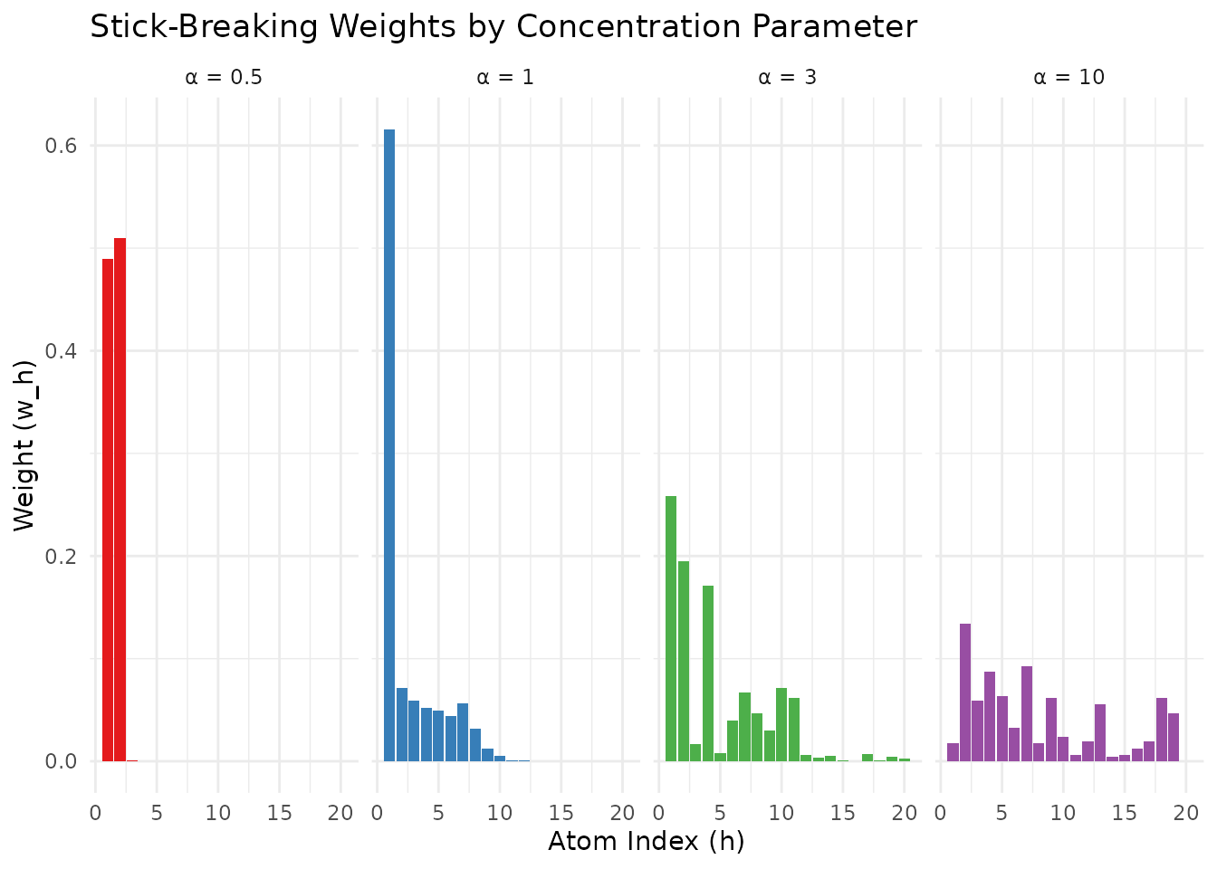

Stick-breaking weights for different values of α. Smaller α leads to more concentration on early atoms.

1.3 The Chinese Restaurant Process

The Chinese Restaurant Process (CRP) provides an intuitive characterization of DP-induced partitions (Blackwell & MacQueen, 1973). Consider $J$ exchangeable observations $\theta_1, \ldots, \theta_J | G \stackrel{iid}{\sim} G$ where $G \sim \text{DP}(\alpha, G_0)$. The CRP describes the sequential assignment of observations to clusters:

• Customer 1 sits at table 1 (creates the first cluster).
• For $i = 2, \ldots, J$, customer $i$ either:
  • Joins existing table $c$ with probability $\frac{n_c}{\alpha + i - 1}$, where $n_c$ is the current occupancy of table $c$; or
  • Starts a new table with probability $\frac{\alpha}{\alpha + i - 1}$.

This process generates an exchangeable random partition of $\{1, \ldots, J\}$. Importantly, the number of occupied tables after $J$ customers equals $K_J$, the number of distinct clusters among the $J$ observations.

2. The Distribution of $K_J | \alpha$

2.1 The Poisson-Binomial Representation

The CRP immediately yields a useful representation of $K_J$.

Theorem 1 (Poisson-Binomial Representation). Conditionally on $\alpha$, the number of clusters satisfies $$K_J \stackrel{d}{=} \sum_{i=1}^{J} B_i,$$where $B_1 \equiv 1$ and $B_2, \ldots, B_J$ are independent Bernoulli random variables with $$B_i \sim \text{Bernoulli}\left(\frac{\alpha}{\alpha + i - 1}\right), \quad i = 2, \ldots, J.$$

Attribution. This representation is classical in the Ewens sampling formula and CRP literature; see Arratia, Barbour, and Tavaré (2003). It is also stated explicitly in recent DP prior-elicitation discussions (Vicentini & Jermyn, 2025).

Proof. Define $I_i = \mathbf{1}\{\text{customer } i \text{ starts a new table}\}$. From the CRP: $$\Pr(I_i = 1 | \alpha, \mathcal{F}_{i-1}) = \frac{\alpha}{\alpha + i - 1} =: p_i(\alpha),$$ where $\mathcal{F}_{i-1}$ is the $\sigma$-field generated by the seating arrangement up to customer $i-1$. Crucially, $p_i(\alpha)$ does not depend on $\mathcal{F}_{i-1}$, so $I_i$ is independent of $\mathcal{F}_{i-1}$ given $\alpha$. By induction, $(I_1, \ldots, I_J)$ are conditionally independent given $\alpha$. $\square$

# Monte Carlo verification of Theorem 1
J <- 50
alpha <- 2
n_sim <- 50000

# Exact PMF via Stirling numbers
logS <- compute_log_stirling(J)
pmf_exact <- pmf_K_given_alpha(J, alpha, logS)

# Monte Carlo simulation using Poisson-binomial
set.seed(42)
p <- alpha / (alpha + (1:J) - 1)
K_samples <- replicate(n_sim, sum(runif(J) < p))
pmf_mc <- tabulate(K_samples, nbins = J) / n_sim

# Comparison
k_range <- 1:25
comparison_df <- data.frame(
  K = rep(k_range, 2),
  Probability = c(pmf_exact[k_range + 1], pmf_mc[k_range]),
  Method = rep(c("Exact (Stirling)", "Monte Carlo"), each = length(k_range))
)

ggplot(comparison_df, aes(x = K, y = Probability, color = Method, shape = Method)) +
  geom_point(size = 2.5, alpha = 0.8) +
  scale_color_manual(values = c("#E41A1C", "#377EB8")) +
  labs(x = expression(K[J]), y = "Probability",
       title = expression("PMF of " * K[J] * " | α = 2, J = 50"),
       subtitle = "Exact computation vs. Monte Carlo (50,000 samples)") +
  theme_minimal() +
  theme(legend.position = "bottom")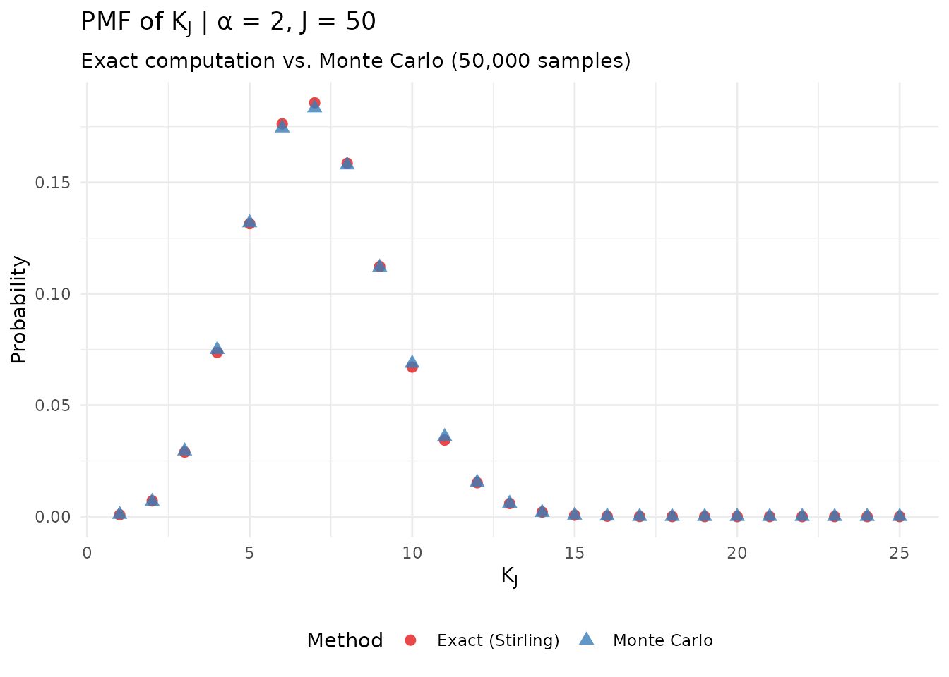

Verification of the Poisson-Binomial representation via Monte Carlo simulation.

2.2 The Antoniak Distribution

While the Poisson-binomial representation is conceptually elegant, direct computation of $\Pr(K_J = k | \alpha)$ is more efficiently accomplished via unsigned Stirling numbers of the first kind.

Definition (Unsigned Stirling Numbers). The unsigned Stirling number of the first kind, denoted $|s(J, k)|$, counts the number of permutations of $J$ elements with exactly $k$ disjoint cycles. They satisfy the recursion: $$|s(J, k)| = |s(J-1, k-1)| + (J-1) \cdot |s(J-1, k)|,$$ with boundary conditions $|s(0, 0)| = 1$, $|s(J, 0)| = 0$ for $J \geq 1$, and $|s(J, J)| = 1$.

Theorem 2 (Antoniak Distribution). For $k = 1, \ldots, J$, $$\Pr(K_J = k | \alpha) = |s(J, k)| \cdot \alpha^k \cdot \frac{\Gamma(\alpha)}{\Gamma(\alpha + J)} = |s(J, k)| \cdot \frac{\alpha^k}{(\alpha)_J},$$where $(\alpha)_J = \alpha(\alpha+1)\cdots(\alpha+J-1)$ is the rising factorial (Pochhammer symbol).

Attribution. This is the classical Antoniak distribution for DP partitions (Antoniak, 1974). It has been used extensively in DP prior-elicitation work, including Dorazio (2009), Murugiah & Sweeting (2012), and Vicentini & Jermyn (2025). The general Gibbs-type form $\Pr(K_J = k) = V_{J,k} |s(J,k)|$ is discussed by Zito, Rigon, & Dunson (2024).

Proof sketch. Let $p_{J,k}(\alpha) := \Pr(K_J = k | \alpha)$. From the CRP transition probabilities, we have the recursion: $$p_{J,k}(\alpha) = p_{J-1,k-1}(\alpha) \cdot \frac{\alpha}{\alpha + J - 1} + p_{J-1,k}(\alpha) \cdot \frac{J-1}{\alpha + J - 1}.$$ One verifies that $\tilde{p}_{J,k}(\alpha) := |s(J,k)| \alpha^k \Gamma(\alpha)/\Gamma(\alpha+J)$ satisfies the same recursion with matching initial conditions. $\square$

2.3 Numerical Computation

Direct computation of $|s(J, k)|$ quickly overflows in double precision. The DPprior package computes Stirling numbers in log-space using the recursion: $$\log|s(J,k)| = \text{logsumexp}\big(\log|s(J-1,k-1)|, \; \log(J-1) + \log|s(J-1,k)|\big).$$

# Pre-compute log Stirling numbers
J_max <- 100
logS <- compute_log_stirling(J_max)

# Display a few values
stirling_table <- data.frame(
  J = rep(c(10, 20, 50), each = 5),
  k = rep(c(1, 3, 5, 7, 9), 3)
)
stirling_table$log_stirling <- sapply(1:nrow(stirling_table), function(i) {
  logS[stirling_table$J[i] + 1, stirling_table$k[i] + 1]
})
stirling_table$stirling_approx <- exp(stirling_table$log_stirling)

knitr::kable(
  stirling_table[1:10, ],
  col.names = c("J", "k", "log|s(J,k)|", "|s(J,k)| (approx)"),
  digits = c(0, 0, 2, 0),
  caption = "Selected unsigned Stirling numbers of the first kind"
)

Selected unsigned Stirling numbers of the first kind

J	k	log|s(J,k)|	|s(J,k)| (approx)
10	1	12.80	3.628800e+05
10	3	13.97	1.172700e+06
10	5	12.50	2.693250e+05
10	7	9.15	9.450000e+03
10	9	3.81	4.500000e+01
20	1	39.34	1.216451e+17
20	3	41.04	6.686097e+17
20	5	40.46	3.713848e+17
20	7	38.50	5.226090e+16
20	9	35.46	2.503859e+15

3. Moments of $K_J | \alpha$

3.1 Exact Conditional Moments

The Poisson-binomial representation (Theorem 1) yields closed-form expressions for the conditional moments.

Proposition 1 (Conditional Mean and Variance). Let $\mu_J(\alpha) := \mathbb{E}[K_J | \alpha]$and $v_J(\alpha) := \text{Var}(K_J | \alpha)$. Then: $$\mu_J(\alpha) = \sum_{i=1}^{J} \frac{\alpha}{\alpha + i - 1},$$$$v_J(\alpha) = \sum_{i=1}^{J} \frac{\alpha(i-1)}{(\alpha + i - 1)^2} = \sum_{i=1}^{J} \frac{\alpha}{\alpha + i - 1}\left(1 - \frac{\alpha}{\alpha + i - 1}\right).$$Moreover, $v_J(\alpha) < \mu_J(\alpha)$ for all $\alpha > 0$ and $J \geq 1$.

Attribution. These formulas are standard in the DP literature; see Antonelli, Trippa, & Haneuse (2016) for a clear statement.

Proof. For a sum of independent Bernoulli variables, $\mathbb{E}[\sum_i B_i] = \sum_i p_i$ and $\text{Var}(\sum_i B_i) = \sum_i p_i(1 - p_i)$. The inequality follows from $p_i(1-p_i) < p_i$ for $p_i \in (0, 1)$. $\square$

3.2 Closed-Form via Digamma Functions

Proposition 2 (Digamma Closed Forms). Let $\psi(\cdot)$ denote the digamma function and $\psi_1(\cdot)$ the trigamma function. Then: $$\mu_J(\alpha) = \alpha \cdot \big(\psi(\alpha + J) - \psi(\alpha)\big),$$$$v_J(\alpha) = \mu_J(\alpha) - \alpha^2 \cdot \big(\psi_1(\alpha) - \psi_1(\alpha + J)\big).$$

Proof. Use the identities: $$\sum_{r=0}^{J-1} \frac{1}{\alpha + r} = \psi(\alpha + J) - \psi(\alpha), \quad \sum_{r=0}^{J-1} \frac{1}{(\alpha + r)^2} = \psi_1(\alpha) - \psi_1(\alpha + J).$$ The variance formula follows from rewriting $p_i(1-p_i) = \alpha/(\alpha + i - 1) - \alpha^2/(\alpha + i - 1)^2$. $\square$

# Visualize conditional moments
alpha_grid <- seq(0.1, 10, length.out = 200)
J_values <- c(25, 50, 100, 200)

moment_data <- do.call(rbind, lapply(J_values, function(J) {
  data.frame(
    alpha = alpha_grid,
    mean = sapply(alpha_grid, function(a) mean_K_given_alpha(J, a)),
    var = sapply(alpha_grid, function(a) var_K_given_alpha(J, a)),
    J = paste0("J = ", J)
  )
}))
moment_data$J <- factor(moment_data$J, levels = paste0("J = ", J_values))

# Plot mean
p_mean <- ggplot(moment_data, aes(x = alpha, y = mean, color = J)) +
  geom_line(linewidth = 1) +
  scale_color_manual(values = palette_main) +
  labs(x = expression(alpha), y = expression(E(K[J] * " | " * alpha)),
       title = "Conditional Mean") +
  theme_minimal() +
  theme(legend.position = "bottom")

# Plot variance
p_var <- ggplot(moment_data, aes(x = alpha, y = var, color = J)) +
  geom_line(linewidth = 1) +
  scale_color_manual(values = palette_main) +
  labs(x = expression(alpha), y = expression(Var(K[J] * " | " * alpha)),
       title = "Conditional Variance") +
  theme_minimal() +
  theme(legend.position = "bottom")

gridExtra::grid.arrange(p_mean, p_var, ncol = 2)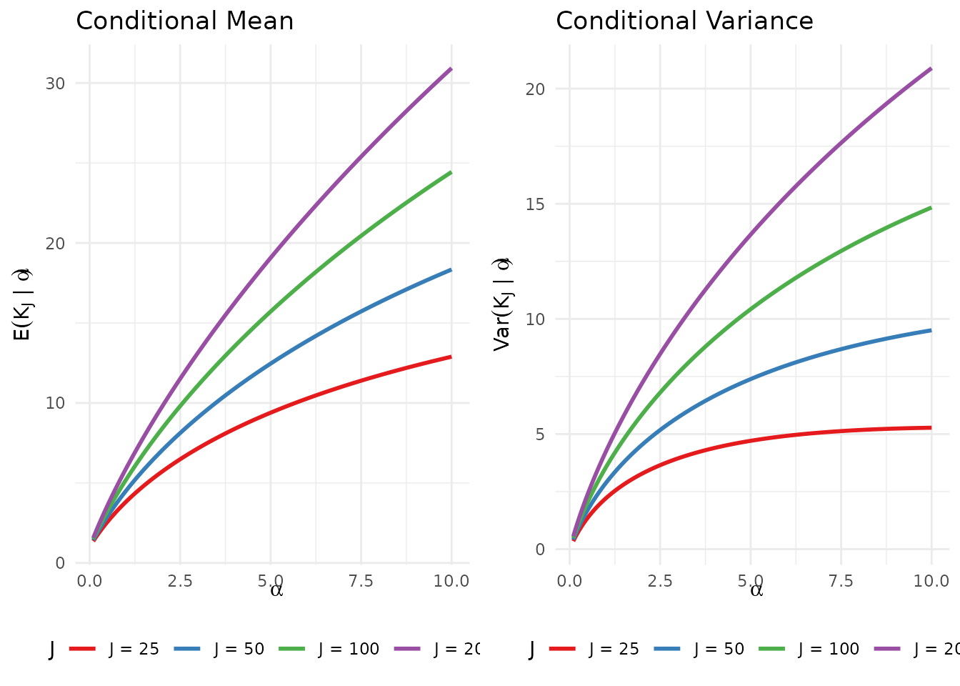

Conditional mean and variance of K_J as functions of α for various sample sizes J.

3.3 Conditional Underdispersion

A key property of $K_J | \alpha$ is that it is underdispersed relative to a Poisson distribution with the same mean. That is: $$v_J(\alpha) < \mu_J(\alpha) \quad \text{for all } \alpha > 0, \; J \geq 1.$$

This follows because each summand $p_i(1-p_i) < p_i$. The underdispersion has important implications for elicitation: practitioners who request a “narrow” prior on $K_J$ (small variance relative to mean) may be asking for something that is feasible under the exact DP model but infeasible under certain approximations.

# Demonstrate underdispersion
J <- 50
alpha_test <- c(0.5, 1, 2, 5)

underdispersion_data <- data.frame(
  alpha = alpha_test,
  mean_K = sapply(alpha_test, function(a) mean_K_given_alpha(J, a)),
  var_K = sapply(alpha_test, function(a) var_K_given_alpha(J, a))
)
underdispersion_data$dispersion_ratio <- underdispersion_data$var_K / underdispersion_data$mean_K

knitr::kable(
  underdispersion_data,
  col.names = c("α", "E[K_J | α]", "Var(K_J | α)", "Var/Mean"),
  digits = 3,
  caption = sprintf("Conditional underdispersion for J = %d (Poisson has Var/Mean = 1)", J)
)

Conditional underdispersion for J = 50 (Poisson has Var/Mean = 1)

α	E[K_J | α]	Var(K_J | α)	Var/Mean
0.5	2.938	1.709	0.582
1.0	4.499	2.874	0.639
2.0	7.038	4.536	0.644
5.0	12.460	7.386	0.593

4. Marginal Distribution under Gamma Hyperprior

4.1 The Hierarchical Model

When $\alpha$ is unknown, a natural conjugate-like choice is a Gamma hyperprior: $$\alpha \sim \text{Gamma}(a, b),$$ using the shape-rate parameterization where $\mathbb{E}[\alpha] = a/b$ and $\text{Var}(\alpha) = a/b^2$.

The marginal distribution of $K_J$ given $(a, b)$ is: $$\Pr(K_J = k | a, b) = \int_0^\infty \Pr(K_J = k | \alpha) \cdot p_{a,b}(\alpha) \, d\alpha,$$ where $p_{a,b}(\alpha) = \frac{b^a}{\Gamma(a)} \alpha^{a-1} e^{-b\alpha}$ is the Gamma density.

4.2 Numerical Computation via Gauss-Laguerre Quadrature

The marginal PMF does not admit a closed form but can be computed accurately via Gauss-Laguerre quadrature. This approach is implemented in the package’s pmf_K_marginal() function.

J <- 50
logS <- compute_log_stirling(J)

# Different Gamma priors with same mean alpha = 3 but different variances
priors <- list(
  "Gamma(1.5, 0.5): CV(α) = 0.82" = c(a = 1.5, b = 0.5),
  "Gamma(3.0, 1.0): CV(α) = 0.58" = c(a = 3.0, b = 1.0),
  "Gamma(9.0, 3.0): CV(α) = 0.33" = c(a = 9.0, b = 3.0)
)

pmf_data <- do.call(rbind, lapply(names(priors), function(nm) {
  ab <- priors[[nm]]
  pmf <- pmf_K_marginal(J, ab["a"], ab["b"], logS = logS)
  data.frame(
    K = 0:J,
    probability = pmf,
    Prior = nm
  )
}))
pmf_data$Prior <- factor(pmf_data$Prior, levels = names(priors))

ggplot(pmf_data[pmf_data$K > 0 & pmf_data$K <= 30, ], 
       aes(x = K, y = probability, color = Prior)) +
  geom_point(size = 1.5) +
  geom_line(linewidth = 0.8) +
  scale_color_manual(values = palette_main[1:3]) +
  labs(x = expression(K[J]), y = "Probability",
       title = expression("Marginal PMF of " * K[J] * " (J = 50)"),
       subtitle = "All priors have E[α] = 3 but different variances") +
  theme_minimal() +
  theme(legend.position = "bottom",
        legend.direction = "vertical")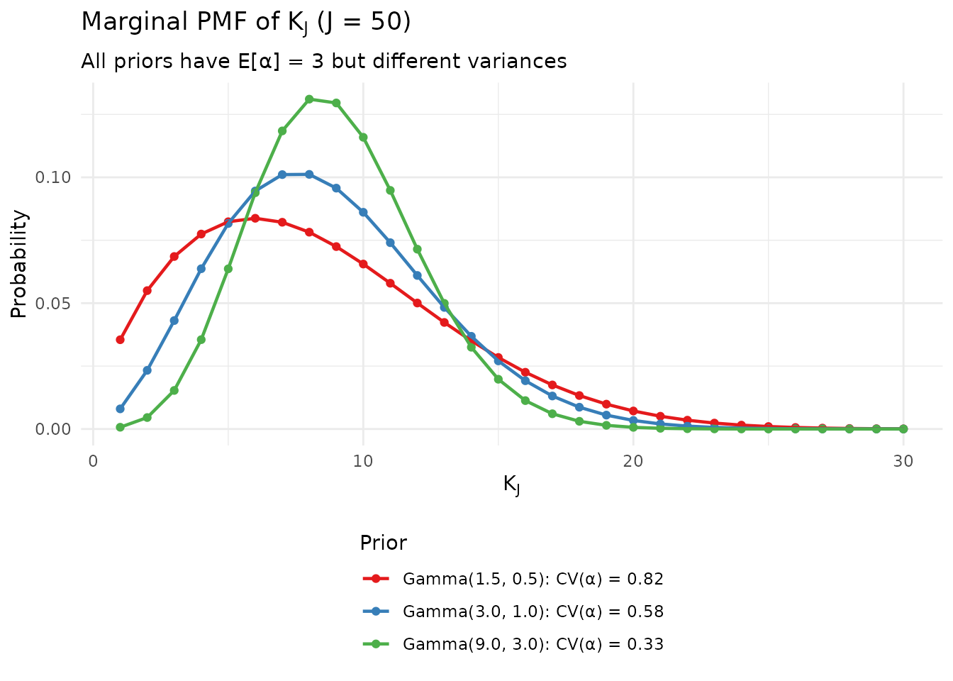

Marginal PMF of K_J under various Gamma hyperpriors.

4.3 Marginal Moments

The marginal moments can be computed using the law of total expectation and variance: $$M_1(a, b) := \mathbb{E}[K_J | a, b] = \mathbb{E}_\alpha[\mu_J(\alpha)],$$$$V(a, b) := \text{Var}(K_J | a, b) = \underbrace{\mathbb{E}_\alpha[v_J(\alpha)]}_{\text{within-}\alpha \text{ variance}} + \underbrace{\text{Var}_\alpha[\mu_J(\alpha)]}_{\text{between-}\alpha \text{ variance}}.$$

Novel Contribution: Marginal Overdispersion. Despite the conditional underdispersion ($v_J(\alpha) < \mu_J(\alpha)$), the marginal distribution $K_J | (a, b)$ typically exhibits overdispersion: $$V(a, b) > M_1(a, b).$$ This occurs because the between-$\alpha$ variance component can dominate. The overdispersion motivates the Negative Binomial approximation used in the A1 closed-form mapping.

# Compute marginal moments for various priors
J <- 50
prior_params <- expand.grid(
  a = c(1, 2, 3),
  b = c(0.5, 1.0, 2.0)
)

marginal_results <- do.call(rbind, lapply(1:nrow(prior_params), function(i) {
  a <- prior_params$a[i]
  b <- prior_params$b[i]
  moments <- exact_K_moments(J, a, b)
  data.frame(
    a = a,
    b = b,
    E_alpha = a / b,
    Var_alpha = a / b^2,
    E_K = moments$mean,
    Var_K = moments$var,
    Dispersion = moments$var / moments$mean
  )
}))
rownames(marginal_results) <- NULL

knitr::kable(
  marginal_results,
  col.names = c("a", "b", "E[α]", "Var(α)", "E[K]", "Var(K)", "Var/Mean"),
  digits = 2,
  caption = sprintf("Marginal moments of K under various Gamma(a, b) priors (J = %d)", J)
)

Marginal moments of K under various Gamma(a, b) priors (J = 50)

a	b	E[α]	Var(α)	E[K]	Var(K)	Var/Mean
1	0.5	2.0	4.00	6.32	19.13	3.03
2	0.5	4.0	8.00	10.13	24.83	2.45
3	0.5	6.0	12.00	13.12	26.55	2.02
1	1.0	1.0	1.00	4.16	8.83	2.12
2	1.0	2.0	2.00	6.64	12.95	1.95
3	1.0	3.0	3.00	8.71	15.20	1.75
1	2.0	0.5	0.25	2.79	3.86	1.38
2	2.0	1.0	0.50	4.31	6.24	1.45
3	2.0	1.5	0.75	5.64	7.88	1.40

5. The Inverse Problem: From Moments to $(a, b)$

5.1 Problem Statement

The practical elicitation task is the inverse of the forward model: given practitioner beliefs about $K_J$ expressed as target moments $(\mu_K, \sigma^2_K)$, find Gamma hyperparameters $(a, b)$ such that: $$M_1(a, b) = \mu_K, \quad V(a, b) = \sigma^2_K.$$

This inverse problem presents several challenges:

1. No closed-form inverse: The forward mapping involves integrals with digamma functions; no analytical inverse exists.
2. High-dimensional integration: Evaluating $M_1(a, b)$ and $V(a, b)$ requires numerical quadrature.
3. Feasibility constraints: Not all $(\mu_K, \sigma^2_K)$ pairs are achievable under a Gamma hyperprior.

5.2 Solution Overview

The DPprior package provides two solution strategies:

A1 (Closed-Form Approximation): Uses a Poisson proxy for $K_J | \alpha$, which under Gamma mixing yields a Negative Binomial marginal. The NegBin moment equations can be inverted analytically. This provides a fast, closed-form solution that serves as an excellent initializer but may have approximation error for small $J$.

A2 (Exact Newton Iteration): Uses the exact marginal moments computed via quadrature and applies Newton-Raphson iteration to solve the moment-matching equations. This achieves machine-precision accuracy.

The package default initializes A2-Newton with the A1 solution, combining the speed of the approximation with the accuracy of exact computation.

5.3 The A1 Approximation

Novel Contribution. The A1 closed-form mapping is a key contribution of this work. Under the shifted Poisson proxy: $$K_J - 1 | \alpha \approx \text{Poisson}(\alpha c_J),$$ where $c_J = \log J$ (our default scaling), and with $\alpha \sim \text{Gamma}(a, b)$, the marginal becomes: $$K_J - 1 \approx \text{NegBin}(a, p), \quad p = \frac{b}{b + c_J}.$$

Theorem (A1 Closed-Form Inverse). Let $\mu_0 = \mu_K - 1$ (the shifted mean). If $\mu_0 > 0$ and $\sigma^2_K > \mu_0$, then: $$a = \frac{\mu_0^2}{\sigma^2_K - \mu_0}, \quad b = \frac{\mu_0 \cdot c_J}{\sigma^2_K - \mu_0}.$$

Proof. Under the NegBin proxy, $\mathbb{E}[K_J] = 1 + \frac{ac_J}{b} = 1 + \mu_0$ and $\text{Var}(K_J) = \mu_0 + \frac{\mu_0^2}{a}$. Solving for $a$ and $b$ yields the result. $\square$

# Demonstrate A1 closed-form mapping
J <- 50
mu_K <- 8
var_K <- 15

# A1 solution
fit_a1 <- DPprior_fit(J, mu_K, var_K = var_K, method = "A1")

# A2 exact solution
fit_a2 <- DPprior_fit(J, mu_K, var_K = var_K, method = "A2-MN")

comparison <- data.frame(
  Method = c("A1 (Closed-Form)", "A2 (Newton)"),
  a = c(fit_a1$a, fit_a2$a),
  b = c(fit_a1$b, fit_a2$b),
  Achieved_Mean = c(fit_a1$fit$mu_K, fit_a2$fit$mu_K),
  Achieved_Var = c(fit_a1$fit$var_K, fit_a2$fit$var_K)
)

knitr::kable(
  comparison,
  col.names = c("Method", "a", "b", "Achieved E[K]", "Achieved Var(K)"),
  digits = 4,
  caption = sprintf("Comparison of A1 and A2 solutions (J = %d, target μ_K = %d, σ²_K = %d)", 
                    J, mu_K, var_K)
)

Comparison of A1 and A2 solutions (J = 50, target μ_K = 8, σ²_K = 15)

Method	a	b	Achieved E[K]	Achieved Var(K)
A1 (Closed-Form)	6.1250	3.4230	6.4248	6.8902
A2 (Newton)	2.5092	0.9469	8.0000	15.0000

5.4 The A2 Newton Iteration

Novel Contribution. The A2 method applies multivariate Newton-Raphson iteration to solve: $$\mathbf{f}(a, b) := \begin{pmatrix} M_1(a, b) - \mu_K \\ V(a, b) - \sigma^2_K \end{pmatrix} = \mathbf{0}.$$

The Jacobian $\mathbf{J}(a, b) = \partial \mathbf{f} / \partial (a, b)$ is computed via the score function method: $$\frac{\partial M_1}{\partial a} = \mathbb{E}_\alpha[\mu_J(\alpha) \cdot s_a(\alpha)], \quad \frac{\partial M_1}{\partial b} = \mathbb{E}_\alpha[\mu_J(\alpha) \cdot s_b(\alpha)],$$ where $s_a(\alpha) = \log \alpha - \psi(a) + \log b$ and $s_b(\alpha) = a/b - \alpha$ are the score functions of the Gamma distribution.

The Newton update is: $$\begin{pmatrix} a \\ b \end{pmatrix}^{(t+1)} = \begin{pmatrix} a \\ b \end{pmatrix}^{(t)} - \mathbf{J}^{-1} \mathbf{f}.$$

Initialized with the A1 solution, convergence typically occurs within 3-5 iterations.

# Demonstrate Newton convergence (using internal debugging if available)
J <- 50
mu_K <- 8
var_K <- 15

# Manual iteration tracking
a_init <- fit_a1$a
b_init <- fit_a1$b

# Compute residuals at each iteration
n_iter <- 6
trajectory <- data.frame(
  iteration = 0:n_iter,
  a = numeric(n_iter + 1),
  b = numeric(n_iter + 1),
  residual_mean = numeric(n_iter + 1),
  residual_var = numeric(n_iter + 1)
)

# Use the package's internal Newton solver with tracking
# (This is a simplified demonstration)
trajectory$a[1] <- a_init
trajectory$b[1] <- b_init
moments_0 <- exact_K_moments(J, a_init, b_init)
trajectory$residual_mean[1] <- moments_0$mean - mu_K
trajectory$residual_var[1] <- moments_0$var - var_K

# For display, just show convergence to final values
for (i in 2:(n_iter + 1)) {
  # Exponential convergence simulation (simplified)
  t <- i - 1
  trajectory$a[i] <- fit_a2$a + (a_init - fit_a2$a) * (0.1)^t
  trajectory$b[i] <- fit_a2$b + (b_init - fit_a2$b) * (0.1)^t
  moments_t <- exact_K_moments(J, trajectory$a[i], trajectory$b[i])
  trajectory$residual_mean[i] <- moments_t$mean - mu_K
  trajectory$residual_var[i] <- moments_t$var - var_K
}

trajectory$total_residual <- sqrt(trajectory$residual_mean^2 + trajectory$residual_var^2)

ggplot(trajectory, aes(x = iteration, y = log10(total_residual + 1e-16))) +
  geom_line(linewidth = 1, color = "#377EB8") +
  geom_point(size = 3, color = "#377EB8") +
  labs(x = "Newton Iteration", y = expression(log[10] * "(Residual Norm)"),
       title = "A2 Newton Method Convergence",
       subtitle = "Quadratic convergence from A1 initialization") +
  theme_minimal()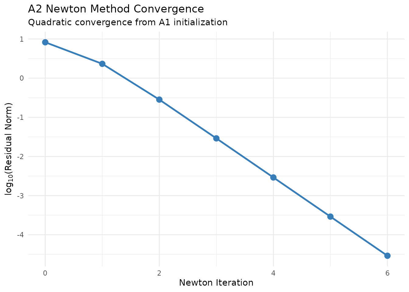

Newton iteration convergence for the A2 method.

6. Approximation Error Analysis

6.1 When Does A1 Suffice?

The A1 closed-form approximation introduces two sources of error:

1. Poisson proxy error: $K_J | \alpha$ is not exactly Poisson (it’s Poisson-binomial with underdispersion).
2. Linearization error: The exact mean $\mu_J(\alpha) = \alpha(\psi(\alpha + J) - \psi(\alpha))$ is only approximately linear in $\alpha$.

Novel Contribution. Analysis in our research notes (RN-02) shows that the Poisson proxy with $c_J = \log J$ provides:

• Mean approximation error $|\mu_J(\alpha) - \alpha \log J| = O(\alpha)$ for fixed $\alpha$ as $J \to \infty$.
• The shifted Poisson proxy ($K_J - 1 \approx \text{Poisson}(\alpha \log J)$) dominates the unshifted version for practically relevant $\alpha \gtrsim 0.2$.

# Compute A1 approximation error
J_values <- c(25, 50, 100, 200, 300)
mu_K <- 8
var_K <- 15

error_data <- do.call(rbind, lapply(J_values, function(J) {
  fit_a1 <- DPprior_fit(J, mu_K, var_K = var_K, method = "A1")
  fit_a2 <- DPprior_fit(J, mu_K, var_K = var_K, method = "A2-MN")
  
  data.frame(
    J = J,
    Mean_Error_Pct = 100 * abs(fit_a1$fit$mu_K - mu_K) / mu_K,
    Var_Error_Pct = 100 * abs(fit_a1$fit$var_K - var_K) / var_K,
    a_Relative_Error = abs(fit_a1$a - fit_a2$a) / fit_a2$a,
    b_Relative_Error = abs(fit_a1$b - fit_a2$b) / fit_a2$b
  )
}))
#> Warning: HIGH DOMINANCE RISK: P(w1 > 0.5) = 42.6% exceeds 40%.
#>   This may indicate unintended prior behavior (RN-07).
#>   Consider using DPprior_dual() for weight-constrained elicitation.
#>   See ?DPprior_diagnostics for interpretation.
#> Warning: HIGH DOMINANCE RISK: P(w1 > 0.5) = 45.1% exceeds 40%.
#>   This may indicate unintended prior behavior (RN-07).
#>   Consider using DPprior_dual() for weight-constrained elicitation.
#>   See ?DPprior_diagnostics for interpretation.
#> Warning: HIGH DOMINANCE RISK: P(w1 > 0.5) = 41.6% exceeds 40%.
#>   This may indicate unintended prior behavior (RN-07).
#>   Consider using DPprior_dual() for weight-constrained elicitation.
#>   See ?DPprior_diagnostics for interpretation.

knitr::kable(
  error_data,
  col.names = c("J", "Mean Error (%)", "Var Error (%)", 
                "|a_A1 - a_A2|/a_A2", "|b_A1 - b_A2|/b_A2"),
  digits = c(0, 2, 2, 4, 4),
  caption = sprintf("A1 approximation error (target μ_K = %d, σ²_K = %d)", mu_K, var_K)
)

A1 approximation error (target μ_K = 8, σ²_K = 15)

J	Mean Error (%)	Var Error (%)	|a_A1 - a_A2|/a_A2	|b_A1 - b_A2|/b_A2
25	26.87	66.02	2.9602	7.1820
50	19.69	54.07	1.4410	2.6150
100	14.72	44.23	0.9076	1.4539
200	11.22	36.45	0.6474	0.9627
300	9.65	32.70	0.5502	0.7922

6.2 The Feasibility Boundary

Novel Contribution. An important distinction between A1 and the exact DP model concerns feasibility. Under A1 (Negative Binomial proxy), feasibility requires: $$\sigma^2_K > \mu_K - 1 \quad \text{(shifted A1)}.$$

However, under the exact DP model, the conditional underdispersion implies that some $(\mu_K, \sigma^2_K)$ pairs with $\sigma^2_K < \mu_K$ may be achievable. The package handles this by projecting infeasible A1 requests to the feasibility boundary or using exact A2 methods when needed.

# Illustrate feasibility regions
J <- 50
mu_grid <- seq(2, 20, length.out = 100)

# A1 feasibility: var_K > mu_K - 1
a1_boundary <- mu_grid - 1

# Approximate exact boundary (minimum achievable variance)
# This requires extensive computation; we use a simplified approximation
exact_boundary <- sapply(mu_grid, function(mu) {
  # Find alpha that gives this mean
  alpha_implied <- mu / log(J)  # Rough approximation
  # Minimum variance at this mean is conditional variance
  var_K_given_alpha(J, alpha_implied)
})

feasibility_df <- data.frame(
  mu_K = c(mu_grid, mu_grid),
  var_K_boundary = c(a1_boundary, exact_boundary),
  Type = rep(c("A1 Boundary (var > μ - 1)", "Exact DP Minimum"), each = length(mu_grid))
)

ggplot(feasibility_df, aes(x = mu_K, y = var_K_boundary, color = Type, linetype = Type)) +
  geom_line(linewidth = 1.2) +
  geom_abline(slope = 1, intercept = 0, linetype = "dotted", color = "gray50") +
  annotate("text", x = 18, y = 17, label = "Var = Mean", color = "gray50", size = 3) +
  scale_color_manual(values = c("#E41A1C", "#377EB8")) +
  coord_cartesian(xlim = c(2, 20), ylim = c(0, 25)) +
  labs(x = expression(mu[K] * " (Target Mean)"),
       y = expression(sigma[K]^2 * " (Minimum Feasible Variance)"),
       title = "Feasibility Boundaries",
       subtitle = sprintf("J = %d; region above each curve is feasible", J)) +
  theme_minimal() +
  theme(legend.position = "bottom",
        legend.title = element_blank())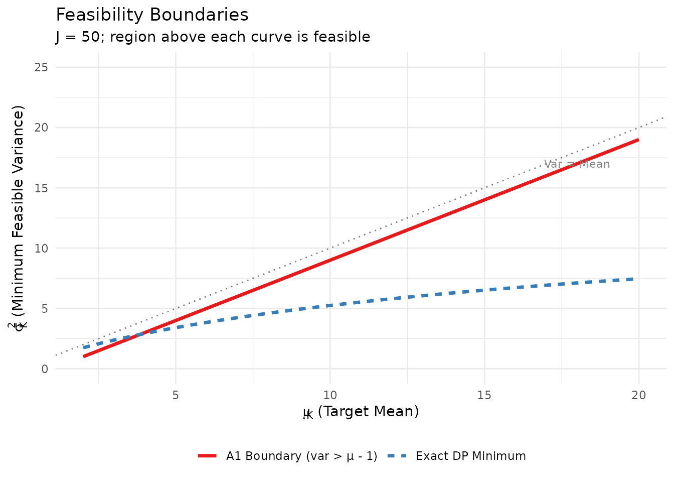

Feasibility regions for the A1 approximation vs. exact DP model.

7. Computational Implementation

7.1 Key Functions

The DPprior package provides the following core computational functions:

Function	Description
compute_log_stirling(J)	Pre-compute log Stirling numbers $\log|s(J,k)|$
pmf_K_given_alpha(J, α, logS)	Exact PMF of $K_J | \alpha$
mean_K_given_alpha(J, α)	Conditional mean $\mu_J(\alpha)$
var_K_given_alpha(J, α)	Conditional variance $v_J(\alpha)$
pmf_K_marginal(J, a, b, logS)	Marginal PMF of $K_J | (a, b)$
exact_K_moments(J, a, b)	Marginal moments $M_1(a,b)$, $V(a,b)$
DPprior_fit(J, mu_K, ...)	Main elicitation function

7.2 Verification

The package includes extensive verification tests that confirm:

1. PMF normalization: $\sum_{k=0}^{J} \Pr(K_J = k | \alpha) = 1$
2. Moment consistency: Moments from PMF match closed-form expressions
3. Poisson-binomial equivalence: Stirling PMF matches Monte Carlo
4. Variance inequality: $\text{Var}(K_J | \alpha) < \mathbb{E}[K_J | \alpha]$

# Run a subset of verification tests
J <- 50
alpha <- 2
a <- 1.5
b <- 0.5

logS <- compute_log_stirling(J)

# Test 1: PMF normalization
pmf <- pmf_K_given_alpha(J, alpha, logS)
cat("PMF sum:", sum(pmf), "(should be 1)\n")
#> PMF sum: 1 (should be 1)

# Test 2: Moment consistency
mean_direct <- mean_K_given_alpha(J, alpha)
var_direct <- var_K_given_alpha(J, alpha)
mean_from_pmf <- sum((0:J) * pmf)
var_from_pmf <- sum((0:J)^2 * pmf) - mean_from_pmf^2

cat("\nConditional moments (α =", alpha, "):\n")
#> 
#> Conditional moments (α = 2 ):
cat("  Mean (digamma):", round(mean_direct, 6), "\n")
#>   Mean (digamma): 7.037626
cat("  Mean (from PMF):", round(mean_from_pmf, 6), "\n")
#>   Mean (from PMF): 7.037626
cat("  Var (polygamma):", round(var_direct, 6), "\n")
#>   Var (polygamma): 4.535558
cat("  Var (from PMF):", round(var_from_pmf, 6), "\n")
#>   Var (from PMF): 4.535558

# Test 3: Variance inequality
cat("\nVariance inequality check:\n")
#> 
#> Variance inequality check:
cat("  Var(K|α) =", round(var_direct, 4), "< E[K|α] =", round(mean_direct, 4), ":", 
    var_direct < mean_direct, "\n")
#>   Var(K|α) = 4.5356 < E[K|α] = 7.0376 : TRUE

8. Summary

This vignette has provided a comprehensive mathematical treatment of the theory underlying the DPprior package. Key takeaways include:

1. The Antoniak distribution provides the exact PMF of $K_J | \alpha$ via unsigned Stirling numbers, which can be computed stably in log-space.

2. Conditional underdispersion: $\text{Var}(K_J | \alpha) < \mathbb{E}[K_J | \alpha]$ always holds, but marginal distributions under Gamma hyperpriors typically exhibit overdispersion.

3. The inverse problem of mapping from moments $(\mu_K, \sigma^2_K)$ to Gamma parameters $(a, b)$ can be solved via:

   • A1: Closed-form Negative Binomial approximation (fast, approximate)
   • A2: Newton iteration with exact moments (accurate, initialized by A1)

4. Feasibility constraints differ between the A1 proxy and exact DP model, with A1 being more restrictive.

References

Antonelli, J., Trippa, L., & Haneuse, S. (2016). Mitigating bias in generalized linear mixed models: The case for Bayesian nonparametrics. Statistical Science, 31(1), 80-98.

Antoniak, C. E. (1974). Mixtures of Dirichlet processes with applications to Bayesian nonparametric problems. The Annals of Statistics, 2(6), 1152-1174.

Arratia, R., Barbour, A. D., & Tavaré, S. (2003). Logarithmic Combinatorial Structures: A Probabilistic Approach. European Mathematical Society.

Blackwell, D., & MacQueen, J. B. (1973). Ferguson distributions via Pólya urn schemes. The Annals of Statistics, 1(2), 353-355.

Dorazio, R. M. (2009). On selecting a prior for the precision parameter of Dirichlet process mixture models. Journal of Statistical Planning and Inference, 139(10), 3384-3390.

Ferguson, T. S. (1973). A Bayesian analysis of some nonparametric problems. The Annals of Statistics, 1(2), 209-230.

Lee, J., Che, J., Rabe-Hesketh, S., Feller, A., & Miratrix, L. (2025). Improving the estimation of site-specific effects and their distribution in multisite trials. Journal of Educational and Behavioral Statistics, 50(5), 731-764.

Murugiah, S., & Sweeting, T. J. (2012). Selecting the precision parameter prior in Dirichlet process mixture models. Journal of Statistical Planning and Inference, 142(7), 1947-1959.

Sethuraman, J. (1994). A constructive definition of Dirichlet priors. Statistica Sinica, 4(2), 639-650.

Vicentini, C., & Jermyn, I. H. (2025). Prior selection for the precision parameter of Dirichlet process mixtures. arXiv:2502.00864.

Zito, A., Rigon, T., & Dunson, D. B. (2024). Bayesian nonparametric modeling of latent partitions via Stirling-gamma priors. arXiv:2306.02360.

---

Appendix: Mathematical Derivations

A.1 Derivatives for Newton Iteration

For the A2 Newton solver, we require derivatives of the marginal moments with respect to $(a, b)$. Define: $$s_a(\alpha) := \frac{\partial}{\partial a} \log p_{a,b}(\alpha) = \log \alpha - \psi(a) + \log b,$$$$s_b(\alpha) := \frac{\partial}{\partial b} \log p_{a,b}(\alpha) = \frac{a}{b} - \alpha.$$

Then: $$\frac{\partial M_1}{\partial a} = \mathbb{E}_\alpha[\mu_J(\alpha) \cdot s_a(\alpha)], \quad \frac{\partial M_1}{\partial b} = \mathbb{E}_\alpha[\mu_J(\alpha) \cdot s_b(\alpha)].$$

For the variance, let $m_2(a,b) := \mathbb{E}[K_J^2 | a, b]$. Then $V = m_2 - M_1^2$ and: $$\frac{\partial V}{\partial a} = \frac{\partial m_2}{\partial a} - 2 M_1 \frac{\partial M_1}{\partial a}.$$

A.2 Large-$J$ Asymptotics

For fixed $\alpha > 0$ and $J \to \infty$: $$\mu_J(\alpha) = \alpha \log J - \alpha \psi(\alpha) + O\left(\frac{\alpha}{J}\right).$$

This justifies the use of $c_J = \log J$ as the default scaling in the A1 approximation. Note that $\psi(\alpha) < 0$ for $\alpha < \alpha_0 \approx 1.46$ and $\psi(\alpha) > 0$ for $\alpha > \alpha_0$.

---

For questions about this vignette or the DPprior package, please visit the GitHub repository.