Beyond Cluster Counts: Dual-Anchor Elicitation for Weight Control
JoonHo Lee
2026-05-07
Source:vignettes/dual-anchor.Rmd
dual-anchor.RmdOverview
The previous vignettes focused on calibrating a Gamma hyperprior for based on your expectations about the number of clusters . This approach is intuitive: you specify how many groups you expect, and the DPprior package finds the corresponding prior on .
However, as Vicentini & Jermyn (2025) have pointed out, matching alone can lead to unintended prior behavior on the cluster weights. Specifically, a prior that produces the “right” expected number of clusters may simultaneously imply a high probability that a single cluster dominates the entire mixture.
This vignette introduces the dual-anchor framework, which allows you to control both:
- Anchor 1: The number of occupied clusters (as before)
- Anchor 2: A weight-related quantity (e.g., or ) that captures how mass is distributed across clusters
By the end of this vignette, you will understand:
- Why K-only calibration can produce surprising weight behavior
- Two key weight anchors: and (co-clustering probability)
- How to use
DPprior_dual()for dual-anchor elicitation - When and how to choose between different anchors and values
1. The Hidden Problem: Unintended Weight Priors
1.1 What K-Only Calibration Misses
Consider a researcher analyzing a multisite educational trial with 50 sites, expecting that treatment effects will cluster into approximately 5 distinct patterns. Using the K-only calibration approach from the Applied Guide, they obtain:
J <- 50
mu_K <- 5

fit_K <- DPprior_fit(J = J, mu_K = mu_K, confidence = "low")
#> Warning: HIGH DOMINANCE RISK: P(w1 > 0.5) = 56.3% exceeds 40%.
#>   This may indicate unintended prior behavior (Lee, 2026).
#>   Consider using DPprior_dual() for weight-constrained elicitation.
#>   See ?DPprior_diagnostics for interpretation.
print(fit_K)
#> DPprior Prior Elicitation Result
#> =============================================
#>
#> Gamma Hyperprior: α ~ Gamma(a = 0.5178, b = 0.3410)
#>   E[α] = 1.519, SD[α] = 2.110
#>
#> Target (J = 50):
#>   E[K_J]   = 5.00
#>   Var(K_J) = 20.00
#>   (from confidence = 'low')
#>
#> Achieved:
#>   E[K_J] = 5.000000, Var(K_J) = 20.000000
#>   Residual = 9.51e-09
#>
#> Method: A2-MN (10 iterations)
#>
#> Dominance Risk: HIGH ✘ (P(w₁>0.5) = 56%)
The fit looks reasonable: the prior expects about 5 clusters with appropriate uncertainty. But what does this prior imply about how mass is distributed across those clusters?
# Examine the implied weight behavior
cat("Weight diagnostics for K-only prior:\n")
#> Weight diagnostics for K-only prior:
cat("  E[w₁] =", round(mean_w1(fit_K$a, fit_K$b), 3), "\n")
#>   E[w₁] = 0.585
cat("  P(w₁ > 0.3) =", round(prob_w1_exceeds(0.3, fit_K$a, fit_K$b), 3), "\n")
#>   P(w₁ > 0.3) = 0.69
cat("  P(w₁ > 0.5) =", round(prob_w1_exceeds(0.5, fit_K$a, fit_K$b), 3), "\n")
#>   P(w₁ > 0.5) = 0.563
cat("  P(w₁ > 0.9) =", round(prob_w1_exceeds(0.9, fit_K$a, fit_K$b), 3), "\n")
#>   P(w₁ > 0.9) = 0.346
Here is the key insight: even though we expect only 5 clusters on average, there is a substantial probability (nearly 50%!) that a randomly selected unit belongs to a cluster containing more than half of all units. This is much more concentrated than many researchers would intuitively expect from “5 clusters.”
1.2 Why Does This Happen?
The relationship between and the cluster weights is not as tight as one might expect. The expected number of clusters follows approximately:
while the expected first stick-breaking weight is:
For and an expected cluster count around 5, we need , which implies . But because is random under our Gamma hyperprior, the tails of the distribution can induce extreme weight behavior: small values lead to close to 1, while large values fragment the weights.
# Illustrate the conditional relationship
alpha_grid <- c(0.5, 1, 2, 5, 10, 20)
w_grid <- seq(0.01, 0.99, length.out = 200)

cond_df <- do.call(rbind, lapply(alpha_grid, function(a) {
  data.frame(
    w = w_grid,
    density = dbeta(w_grid, 1, a),
    alpha = paste0("α = ", a)
  )
}))
cond_df$alpha <- factor(cond_df$alpha, levels = paste0("α = ", alpha_grid))

ggplot(cond_df, aes(x = w, y = density, color = alpha)) +
  geom_line(linewidth = 0.8) +
  scale_color_viridis_d(option = "plasma", end = 0.85) +
  labs(
    x = expression(w[1]),
    y = "Conditional Density",
    title = expression("Conditional Distribution of " * w[1] * " | " * alpha),
    color = NULL
  ) +
  theme_minimal() +
  theme(legend.position = "right")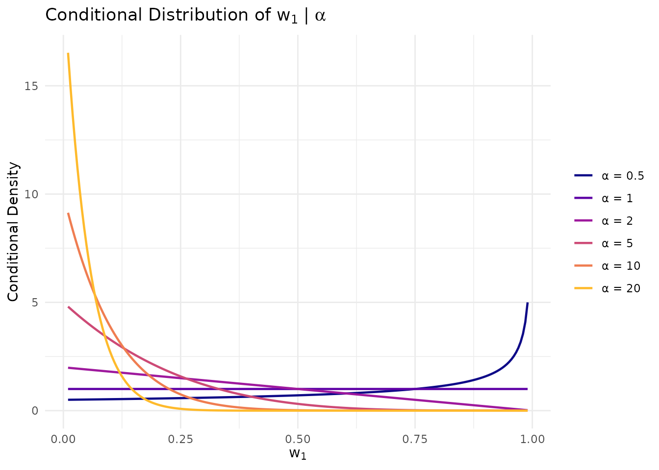
When α is small, w₁ concentrates near 1; when α is large, w₁ concentrates near 0. A diffuse prior on α spans both extremes.
2. Understanding Weight Distributions
Before diving into dual-anchor calibration, let us examine the two weight anchors available in the DPprior package.
2.1 Stick-Breaking Weights Refresher
Under Sethuraman’s stick-breaking representation of the Dirichlet Process, the random mixing measure is:
where the weights are constructed via:
The sequence follows the GEM() distribution and is in size-biased order, not ranked by magnitude.
2.2 Anchor 2a: The First Stick-Breaking Weight ()
The first weight has a particularly tractable distribution. Conditionally, .
Under the hyperprior , the marginal distribution of has fully closed-form expressions:
CDF:
Quantile function:
Survival function (dominance risk):
Important interpretability caveat: is in GEM (size-biased) order, not the largest cluster weight. A faithful interpretation is:
“ is the asymptotic proportion of the cluster containing a randomly selected unit.”
This is still a meaningful dominance diagnostic—if is high, then a randomly selected unit is likely to belong to a cluster that contains more than half the population.
# Using the closed-form w1 functions
a <- fit_K$a
b <- fit_K$b

cat("w₁ distribution under K-only prior:\n")
#> w₁ distribution under K-only prior:
cat("  Mean:     ", round(mean_w1(a, b), 4), "\n")
#>   Mean:      0.5854
cat("  Variance: ", round(var_w1(a, b), 4), "\n")
#>   Variance:  0.1331
cat("  Median:   ", round(quantile_w1(0.5, a, b), 4), "\n")
#>   Median:    0.6169
cat("  90th %ile:", round(quantile_w1(0.9, a, b), 4), "\n")
#>   90th %ile: 1
cat("\nDominance risk:\n")
#>
#> Dominance risk:
cat("  P(w₁ > 0.3):", round(prob_w1_exceeds(0.3, a, b), 4), "\n")
#>   P(w₁ > 0.3): 0.6903
cat("  P(w₁ > 0.5):", round(prob_w1_exceeds(0.5, a, b), 4), "\n")
#>   P(w₁ > 0.5): 0.563
cat("  P(w₁ > 0.9):", round(prob_w1_exceeds(0.9, a, b), 4), "\n")
#>   P(w₁ > 0.9): 0.3463
2.3 Anchor 2b: Co-Clustering Probability ()
The co-clustering probability is defined as:
This has a natural interpretation: equals the probability that two randomly selected units belong to the same cluster. This may be more intuitive for applied researchers to elicit.
The conditional moments are simple:
Note that , so their means are equal, but their full distributions differ.
# Using the rho (co-clustering) functions
cat("Co-clustering probability ρ under K-only prior:\n")
#> Co-clustering probability ρ under K-only prior:
cat("  E[ρ]:     ", round(mean_rho(a, b), 4), "\n")
#>   E[ρ]:      0.5854
cat("  Var(ρ):   ", round(var_rho(a, b), 6), "\n")
#>   Var(ρ):    0.107831
cat("  SD(ρ):    ", round(sqrt(var_rho(a, b)), 4), "\n")
#>   SD(ρ):     0.3284

# Compare with w1
cat("\nNote: E[w₁] = E[ρ] =", round(mean_w1(a, b), 4), "\n")
#>
#> Note: E[w₁] = E[ρ] = 0.5854
cat("But: Var(w₁) =", round(var_w1(a, b), 4), "≠ Var(ρ) =",
    round(var_rho(a, b), 6), "\n")
#> But: Var(w₁) = 0.1331 ≠ Var(ρ) = 0.107831
3. The Dual-Anchor Framework
3.1 The Core Idea
The dual-anchor framework finds Gamma hyperparameters that satisfy two types of constraints simultaneously:
- Anchor 1: Match your beliefs about (number of clusters)
- Anchor 2: Match your beliefs about a weight quantity
This is formalized as an optimization problem:
where measures the discrepancy from the K target and measures the discrepancy from the weight target.
3.2 The Role of
The parameter controls the trade-off between the two anchors:
| Value | Interpretation |
|---|---|
| K-only calibration (ignores weight anchor) | |
| Weight-only calibration (ignores K anchor) | |
| K remains primary, weight provides secondary control | |
| Weight becomes primary (rare in practice) |
In most applications, we recommend , keeping the cluster count as the primary anchor while using the weight constraint to avoid unintended dominance behavior.
3.3 Loss Types: Balancing the Two Anchors
A critical implementation detail is how to scale the two
loss components. The DPprior_dual() function offers three
loss_type options:
loss_type |
Description | When to Use |
|---|---|---|
"relative" |
Normalizes losses by their baseline values | Default; good balance |
"adaptive" |
Estimates scale factors from anchor extremes | More aggressive weight control |
"absolute" |
Raw squared errors (not recommended) | Legacy; scale mismatch issues |
Why does this matter? The K-anchor loss and
weight-anchor loss are measured in different units. Without proper
scaling, the optimizer may effectively ignore one of the anchors. The
"adaptive" option is particularly useful when you want
to produce a meaningful compromise between the two anchors.
4. Using DPprior_dual() for Dual-Anchor
Elicitation
The DPprior_dual() function refines a K-calibrated prior
to also satisfy weight constraints.
4.1 Basic Usage: Probability Constraint
Suppose you want to ensure that the probability of extreme dominance is limited. Specifically, you want :
# Step 1: Start with K-only calibration
fit_K <- DPprior_fit(J = 50, mu_K = 5, confidence = "low")
#> Warning: HIGH DOMINANCE RISK: P(w1 > 0.5) = 56.3% exceeds 40%.
#>   This may indicate unintended prior behavior (Lee, 2026).
#>   Consider using DPprior_dual() for weight-constrained elicitation.
#>   See ?DPprior_diagnostics for interpretation.

cat("K-only prior:\n")
#> K-only prior:
cat("  Gamma(", round(fit_K$a, 3), ",", round(fit_K$b, 3), ")\n")
#>   Gamma( 0.518 , 0.341 )
cat("  P(w₁ > 0.5) =", round(prob_w1_exceeds(0.5, fit_K$a, fit_K$b), 3), "\n\n")
#>   P(w₁ > 0.5) = 0.563

# Step 2: Apply dual-anchor constraint with adaptive loss
fit_dual <- DPprior_dual(
  fit = fit_K,
  w1_target = list(prob = list(threshold = 0.5, value = 0.25)),
  lambda = 0.7,
  loss_type = "adaptive",  # More aggressive weight control
  verbose = FALSE
)

cat("Dual-anchor prior (adaptive):\n")
#> Dual-anchor prior (adaptive):
cat("  Gamma(", round(fit_dual$a, 3), ",", round(fit_dual$b, 3), ")\n")
#>   Gamma( 1.403 , 0.626 )
cat("  P(w₁ > 0.5) =", round(prob_w1_exceeds(0.5, fit_dual$a, fit_dual$b), 3), "\n")
#>   P(w₁ > 0.5) = 0.351
Let us visualize the effect on both the and distributions:
# Prepare data for visualization
logS <- compute_log_stirling(J)

# K distributions
k_grid <- 1:20
k_df <- data.frame(
  K = rep(k_grid, 2),
  probability = c(
    pmf_K_marginal(J, fit_K$a, fit_K$b, logS = logS)[k_grid],
    pmf_K_marginal(J, fit_dual$a, fit_dual$b, logS = logS)[k_grid]
  ),
  Prior = rep(c("K-only", "Dual-anchor"), each = length(k_grid))
)

# w1 distributions
w_grid <- seq(0.01, 0.95, length.out = 200)
w_df <- data.frame(
  w1 = rep(w_grid, 2),
  density = c(
    density_w1(w_grid, fit_K$a, fit_K$b),
    density_w1(w_grid, fit_dual$a, fit_dual$b)
  ),
  Prior = rep(c("K-only", "Dual-anchor"), each = length(w_grid))
)

# Create plots
p1 <- ggplot(k_df, aes(x = K, y = probability, color = Prior)) +
  geom_point(size = 1.5) +
  geom_line(linewidth = 0.8) +
  scale_color_manual(values = palette_2) +
  labs(x = "Number of Clusters (K)", y = "Probability",
       title = "Marginal PMF of K") +
  theme_minimal() +
  theme(legend.position = "bottom")

p2 <- ggplot(w_df, aes(x = w1, y = density, color = Prior)) +
  geom_line(linewidth = 1) +
  geom_vline(xintercept = 0.5, linetype = "dashed", color = "gray50") +
  scale_color_manual(values = palette_2) +
  labs(x = expression(w[1]), y = "Density",
       title = expression("Marginal Density of " * w[1])) +
  theme_minimal() +
  theme(legend.position = "bottom")

gridExtra::grid.arrange(p1, p2, ncol = 2)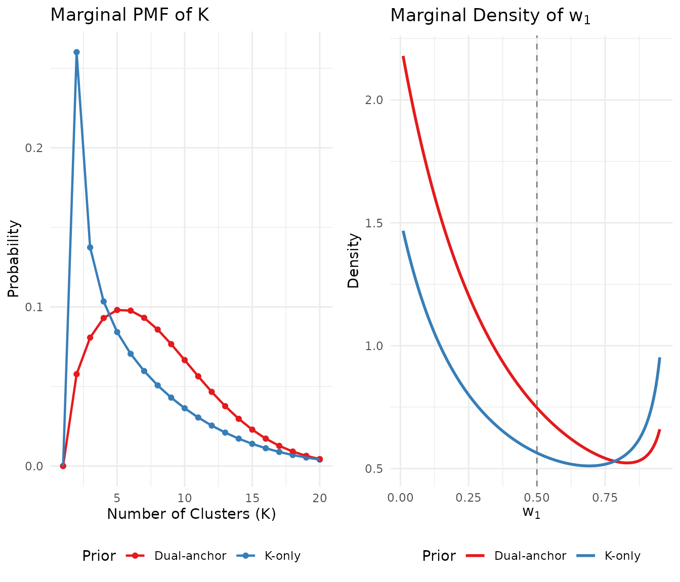
Comparison of K-only vs dual-anchor priors: the dual-anchor approach shifts mass away from extreme w₁ values while maintaining similar K expectations.
4.2 Comparing Loss Types
The choice of loss_type can significantly affect the
results. Let us compare the three options:
# Compare loss types at lambda = 0.5
w1_target <- list(prob = list(threshold = 0.5, value = 0.25))

fit_relative <- DPprior_dual(
  fit_K, w1_target, lambda = 0.5,
  loss_type = "relative", verbose = FALSE
)

fit_adaptive <- DPprior_dual(
  fit_K, w1_target, lambda = 0.5,
  loss_type = "adaptive", verbose = FALSE
)

# Create comparison table
loss_compare <- data.frame(
  Method = c("K-only", "Relative", "Adaptive"),
  a = c(fit_K$a, fit_relative$a, fit_adaptive$a),
  b = c(fit_K$b, fit_relative$b, fit_adaptive$b),
  E_K = c(
    exact_K_moments(J, fit_K$a, fit_K$b)$mean,
    exact_K_moments(J, fit_relative$a, fit_relative$b)$mean,
    exact_K_moments(J, fit_adaptive$a, fit_adaptive$b)$mean
  ),
  P_w1_gt_50 = c(
    prob_w1_exceeds(0.5, fit_K$a, fit_K$b),
    prob_w1_exceeds(0.5, fit_relative$a, fit_relative$b),
    prob_w1_exceeds(0.5, fit_adaptive$a, fit_adaptive$b)
  )
)

loss_compare$a <- round(loss_compare$a, 3)
loss_compare$b <- round(loss_compare$b, 3)
loss_compare$E_K <- round(loss_compare$E_K, 2)
loss_compare$P_w1_gt_50 <- round(loss_compare$P_w1_gt_50, 3)

knitr::kable(
  loss_compare,
  col.names = c("Method", "a", "b", "E[K]", "P(w₁>0.5)"),
  caption = "Comparison of loss types at λ = 0.5 (target: P(w₁>0.5) = 0.25)"
)| Method | a | b | E[K] | P(w₁>0.5) |
|---|---|---|---|---|
| K-only | 0.518 | 0.341 | 5.00 | 0.563 |
| Relative | 0.736 | 0.424 | 5.63 | 0.490 |
| Adaptive | 1.737 | 0.715 | 7.43 | 0.308 |
The "adaptive" loss type typically produces more
noticeable weight reduction because it normalizes each loss component by
its scale at the opposite anchor’s optimum.
4.3 Alternative: Quantile Constraint
You can also specify a quantile constraint. For example, to ensure that the 90th percentile of does not exceed 0.6:
fit_dual_q <- DPprior_dual(
  fit = fit_K,
  w1_target = list(quantile = list(prob = 0.9, value = 0.6)),
  lambda = 0.7,
  loss_type = "adaptive",
  verbose = FALSE
)

cat("Dual-anchor (quantile constraint):\n")
#> Dual-anchor (quantile constraint):
cat("  Gamma(", round(fit_dual_q$a, 3), ",", round(fit_dual_q$b, 3), ")\n")
#>   Gamma( 0.518 , 0.341 )
cat("  90th percentile of w₁:", round(quantile_w1(0.9, fit_dual_q$a, fit_dual_q$b), 3), "\n")
#>   90th percentile of w₁: 1
cat("  (Target was 0.6)\n")
#>   (Target was 0.6)
4.4 Alternative: Mean Constraint
For constraints based on :
fit_dual_m <- DPprior_dual(
  fit = fit_K,
  w1_target = list(mean = 0.35),
  lambda = 0.6,
  loss_type = "adaptive",
  verbose = FALSE
)

cat("Dual-anchor (mean constraint):\n")
#> Dual-anchor (mean constraint):
cat("  Gamma(", round(fit_dual_m$a, 3), ",", round(fit_dual_m$b, 3), ")\n")
#>   Gamma( 1.377 , 0.621 )
cat("  E[w₁]:", round(mean_w1(fit_dual_m$a, fit_dual_m$b), 3), "\n")
#>   E[w₁]: 0.411
cat("  (Target was 0.35)\n")
#>   (Target was 0.35)
5. Elicitation Questions for Weight Anchors
Translating substantive knowledge into weight constraints requires careful framing. Here are suggested elicitation questions:
For (Size-Biased Weight)
These questions focus on what happens when you randomly sample a unit:
“If you randomly select a site from your study, what proportion of all sites would you expect to share its effect pattern? What’s a reasonable median estimate?”
“Is there a significant chance (say, > 30%) that a randomly selected site belongs to an effect group that contains more than half of all sites?”
For (Co-Clustering Probability)
These questions may be more intuitive for many researchers:
“If you pick two sites at random, what’s the probability that they belong to the same effect group?”
“How likely is it that any two randomly chosen sites would show substantively similar treatment effects?”
Translation Examples
| Elicited Belief | Formal Constraint |
|---|---|
| “Randomly selected site’s group is ~25% of total (median)” | quantile = list(prob = 0.5, value = 0.25) |
| “Unlikely (≤20%) that random site is in a dominant (>50%) group” | prob = list(threshold = 0.5, value = 0.2) |
| “Two random sites have ~20% chance of same group” | Use anchor with target mean 0.2 |
6. Exploring the Trade-off: Sensitivity
Different values of produce different trade-offs between matching the K anchor and the weight anchor. Let us explore this systematically:
lambda_grid <- c(1.0, 0.9, 0.7, 0.5, 0.3)
w1_target <- list(prob = list(threshold = 0.5, value = 0.2))

lambda_results <- lapply(lambda_grid, function(lam) {
  if (lam == 1.0) {
    # lambda = 1 just returns K-only
    fit <- fit_K
    fit$dual_anchor <- list(lambda = 1.0)
  } else {
    fit <- DPprior_dual(fit_K, w1_target, lambda = lam,
                        loss_type = "adaptive", verbose = FALSE)
  }

  list(
    lambda = lam,
    a = fit$a,
    b = fit$b,
    E_K = exact_K_moments(J, fit$a, fit$b)$mean,
    P_w1_gt_50 = prob_w1_exceeds(0.5, fit$a, fit$b),
    E_w1 = mean_w1(fit$a, fit$b)
  )
})

# Create comparison table
lambda_df <- do.call(rbind, lapply(lambda_results, function(r) {
  data.frame(
    lambda = r$lambda,
    a = round(r$a, 3),
    b = round(r$b, 3),
    E_K = round(r$E_K, 2),
    P_w1_gt_50 = round(r$P_w1_gt_50, 3),
    E_w1 = round(r$E_w1, 3)
  )
}))

knitr::kable(
  lambda_df,
  col.names = c("λ", "a", "b", "E[K]", "P(w₁>0.5)", "E[w₁]"),
  caption = "Effect of λ on dual-anchor calibration (target: P(w₁>0.5) = 0.2, adaptive loss)"
)| λ | a | b | E[K] | P(w₁>0.5) | E[w₁] |
|---|---|---|---|---|---|
| 1.0 | 0.518 | 0.341 | 5.00 | 0.563 | 0.585 |
| 0.9 | 1.032 | 0.520 | 6.31 | 0.417 | 0.460 |
| 0.7 | 1.658 | 0.694 | 7.33 | 0.317 | 0.381 |
| 0.5 | 2.143 | 0.819 | 7.87 | 0.269 | 0.344 |
| 0.3 | 2.597 | 0.933 | 8.26 | 0.236 | 0.320 |
# Visualize the trade-off
tradeoff_df <- data.frame(
  lambda = sapply(lambda_results, `[[`, "lambda"),
  E_K = sapply(lambda_results, `[[`, "E_K"),
  P_w1 = sapply(lambda_results, `[[`, "P_w1_gt_50")
)

ggplot(tradeoff_df, aes(x = E_K, y = P_w1)) +
  geom_path(color = "gray50", linewidth = 0.8) +
  geom_point(aes(color = factor(lambda)), size = 4) +
  geom_hline(yintercept = 0.2, linetype = "dashed", color = "#E41A1C", alpha = 0.7) +
  geom_vline(xintercept = 5, linetype = "dashed", color = "#377EB8", alpha = 0.7) +
  annotate("text", x = 4.7, y = 0.22, label = "w₁ target", hjust = 1, color = "#E41A1C") +
  annotate("text", x = 5.1, y = 0.45, label = "K target", hjust = 0, color = "#377EB8") +
  scale_color_viridis_d(option = "viridis", begin = 0.2, end = 0.8) +
  labs(
    x = "E[K] (Cluster Count)",
    y = expression(P(w[1] > 0.5)),
    title = "Trade-off Between K and Weight Anchors",
    color = "λ"
  ) +
  theme_minimal() +
  theme(legend.position = "right")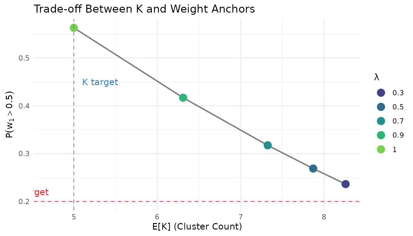
Trade-off curve: reducing λ brings P(w₁ > 0.5) closer to target at the cost of K deviation.
7. Practical Recommendations
7.1 When to Use Dual-Anchor Calibration
Consider dual-anchor calibration when:
High dominance risk in K-only fit: If
print(fit)shows “Dominance Risk: HIGH” orStrong prior belief against concentration: You believe effects should be reasonably spread across groups, not concentrated
Low-information settings: When the data may not strongly update the prior, unintended weight behavior can persist to the posterior
Do not use dual-anchor when:
- You are comfortable with the weight implications of your K-only prior
- You have strong data that will overwhelm any prior specification
- The additional complexity is not justified for your application
7.2 Choosing loss_type
loss_type |
When to Use |
|---|---|
"relative" |
Default choice; balanced trade-off |
"adaptive" |
When you want to give meaningful weight reduction |
"absolute" |
Not recommended (legacy) |
We generally recommend "adaptive" for most dual-anchor
applications, as it ensures that both anchors contribute meaningfully to
the optimization.
8. When Dual-Anchor Constraints Are Infeasible
Not all combinations of K and weight targets are achievable. If you specify conflicting constraints, the optimization may not fully satisfy both:
# An aggressive weight target that conflicts with K target
fit_aggressive <- DPprior_dual(
  fit = fit_K,
  w1_target = list(prob = list(threshold = 0.5, value = 0.05)),  # Very tight
  lambda = 0.5,
  loss_type = "adaptive",
  verbose = FALSE
)

cat("Aggressive dual-anchor attempt:\n")
#> Aggressive dual-anchor attempt:
cat("  Target: P(w₁ > 0.5) = 0.05\n")
#>   Target: P(w₁ > 0.5) = 0.05
cat("  Achieved: P(w₁ > 0.5) =",
    round(prob_w1_exceeds(0.5, fit_aggressive$a, fit_aggressive$b), 3), "\n")
#>   Achieved: P(w₁ > 0.5) = 0.149
cat("\n  Target: E[K] = 5\n")
#>
#>   Target: E[K] = 5
cat("  Achieved: E[K] =",
    round(exact_K_moments(J, fit_aggressive$a, fit_aggressive$b)$mean, 2), "\n")
#>   Achieved: E[K] = 9.41
When constraints are too strict, consider:
Relaxing one of the targets: Accept somewhat higher dominance risk or a different K expectation
Adjusting : If one target is more important, weight it more heavily
Using a single anchor: Sometimes K-only or weight-only calibration is more appropriate
Summary
| Concept | Key Point |
|---|---|
| K-only calibration | May induce unintended weight behavior |
| (first weight) | Size-biased cluster mass; closed-form distribution |
| (co-clustering) | P(two random units share a cluster); intuitive |
loss_type |
Use "adaptive" for meaningful trade-offs |
| Dual-anchor objective | Trade-off between K fit and weight fit via |
| Recommended workflow | 1. K-only fit → 2. Check diagnostics → 3. Dual-anchor if needed |
What’s Next?
Diagnostics: Deep dive into verifying your prior meets specifications
Case Studies: Real-world examples applying dual-anchor calibration
Mathematical Foundations: Theoretical details of the DPprior framework
References
Vicentini, S., & Jermyn, I. H. (2025). Prior selection for the precision parameter of Dirichlet process mixture models. arXiv:2502.00864. https://doi.org/10.48550/arXiv.2502.00864
Sethuraman, J. (1994). A constructive definition of Dirichlet priors. Statistica Sinica, 4(2), 639–650.
For questions or feedback, please visit the GitHub repository.