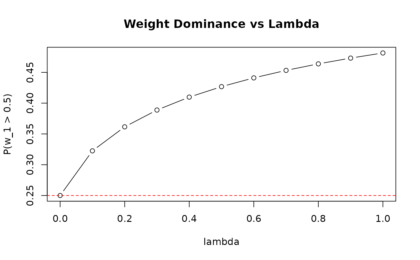
Compute Pareto Trade-off Curve — compute_tradeoff

Explores the trade-off between K_J fit and first-weight constraint over lambda values.

Usage

compute_tradeoff_curve(
  J,
  K_target,
  w1_target,
  lambda_seq = seq(0, 1, by = 0.1),
  max_iter = 100L,
  M = .QUAD_NODES_DEFAULT,
  verbose = FALSE,
  loss_type = c("relative", "adaptive", "absolute")
)

Arguments

J: Integer; sample size.
K_target: List with mu_K and var_K.
w1_target: Weight target specification.
lambda_seq: Numeric vector of lambda values.
max_iter: Integer; max iterations per optimization.
M: Integer; quadrature nodes.
verbose: Logical; print progress.
loss_type: Character; "relative", "adaptive", or "absolute".

Value

Data frame with columns: lambda, a, b, mu_K, var_K, K_loss, w_loss, w1_prob_gt_50, E_w1.

Examples

curve <- compute_tradeoff_curve(
  J = 50,
  K_target = list(mu_K = 5, var_K = 8),
  w1_target = list(prob = list(threshold = 0.5, value = 0.25)),
  lambda_seq = seq(0, 1, by = 0.1),
  loss_type = "relative"
)

# Visualize trade-off
plot(curve$lambda, curve$w1_prob_gt_50, type = "b",
     xlab = "lambda", ylab = "P(w_1 > 0.5)",
     main = "Weight Dominance vs Lambda")
abline(h = 0.25, lty = 2, col = "red")  # target

References

Lee, J. (2026). Design-Conditional Prior Elicitation for Dirichlet Process Mixtures. arXiv preprint arXiv:2602.06301.