The Applied Researcher's Guide to Cluster-Count Elicitation

Overview

This vignette provides a comprehensive, step-by-step guide to eliciting Gamma hyperpriors for the concentration parameter $\alpha$ in Dirichlet Process mixture models. By the end of this guide, you will understand:

The two-question protocol for systematic prior elicitation
How to translate domain knowledge into the expected number of clusters
How to express your uncertainty about that expectation
When to use different calibration methods (A1, A2-MN, A2-KL)
How to handle feasibility constraints
How to conduct sensitivity analysis

This guide assumes you have read the Quick Start vignette and are familiar with the basic usage of DPprior_fit().

1. The Elicitation Framework

The Two-Question Protocol

Eliciting a Gamma $(a, b)$ hyperprior for $\alpha$ requires specifying two pieces of information: a location (where you expect the number of clusters to be) and a scale (how certain you are about that expectation). The DPprior package operationalizes this through two quantities:

Expected number of clusters ( $\mu_K$ ): Your best guess for the number of distinct groups
Uncertainty about that expectation ( $\sigma^2_K$ or a confidence level): How sure you are about your guess

Why do we need both? The Gamma distribution has two parameters, so a single piece of information is insufficient to uniquely determine the prior. Think of it this way: saying “I expect 15 clusters” could correspond to many different priors—from a tightly concentrated prior that strongly believes in exactly 15 clusters, to a diffuse prior that merely centers around 15 but allows for substantial deviation.

# Compare priors with same mean but different variances
J <- 100
mu_K <- 15

fits <- list(
  "High Uncertainty (var_K = 70)"   = DPprior_fit(J, mu_K, var_K = 70),
  "Medium Uncertainty (var_K = 35)" = DPprior_fit(J, mu_K, var_K = 35),
  "Low Uncertainty (var_K = 21)"    = DPprior_fit(J, mu_K, var_K = 21)
)

# Pre-compute log Stirling numbers for PMF calculation
logS <- compute_log_stirling(J)

# Create data for alpha prior plot
alpha_grid <- seq(0.01, 20, length.out = 300)
alpha_df <- do.call(rbind, lapply(names(fits), function(nm) {
  fit <- fits[[nm]]
  data.frame(
    alpha = alpha_grid,
    density = dgamma(alpha_grid, shape = fit$a, rate = fit$b),
    Uncertainty = nm
  )
}))
alpha_df$Uncertainty <- factor(alpha_df$Uncertainty, levels = names(fits))

# Create data for K PMF plot
k_df <- do.call(rbind, lapply(names(fits), function(nm) {
  fit <- fits[[nm]]
  pmf <- pmf_K_marginal(J, fit$a, fit$b, logS = logS)
  data.frame(
    K = 1:length(pmf),
    probability = pmf,
    Uncertainty = nm
  )
}))
k_df$Uncertainty <- factor(k_df$Uncertainty, levels = names(fits))

# Plot alpha priors
p1 <- ggplot(alpha_df, aes(x = alpha, y = density, color = Uncertainty)) +
  geom_line(linewidth = 1) +
  scale_color_manual(values = palette_3) +
  labs(x = expression(alpha), y = "Density",
       title = expression("Prior Density for " * alpha)) +
  theme_minimal() +
  theme(legend.position = "bottom",
        legend.title = element_blank(),
        legend.direction = "vertical")

# Plot K PMF
p2 <- ggplot(k_df[k_df$K <= 35, ], aes(x = K, y = probability, color = Uncertainty)) +
  geom_point(size = 1.5) +
  geom_line(linewidth = 0.8) +
  scale_color_manual(values = palette_3) +
  labs(x = "Number of Clusters (K)", y = "Probability",
       title = "Implied PMF of K") +
  theme_minimal() +
  theme(legend.position = "bottom",
        legend.title = element_blank(),
        legend.direction = "vertical")

# Arrange plots side by side
gridExtra::grid.arrange(p1, p2, ncol = 2)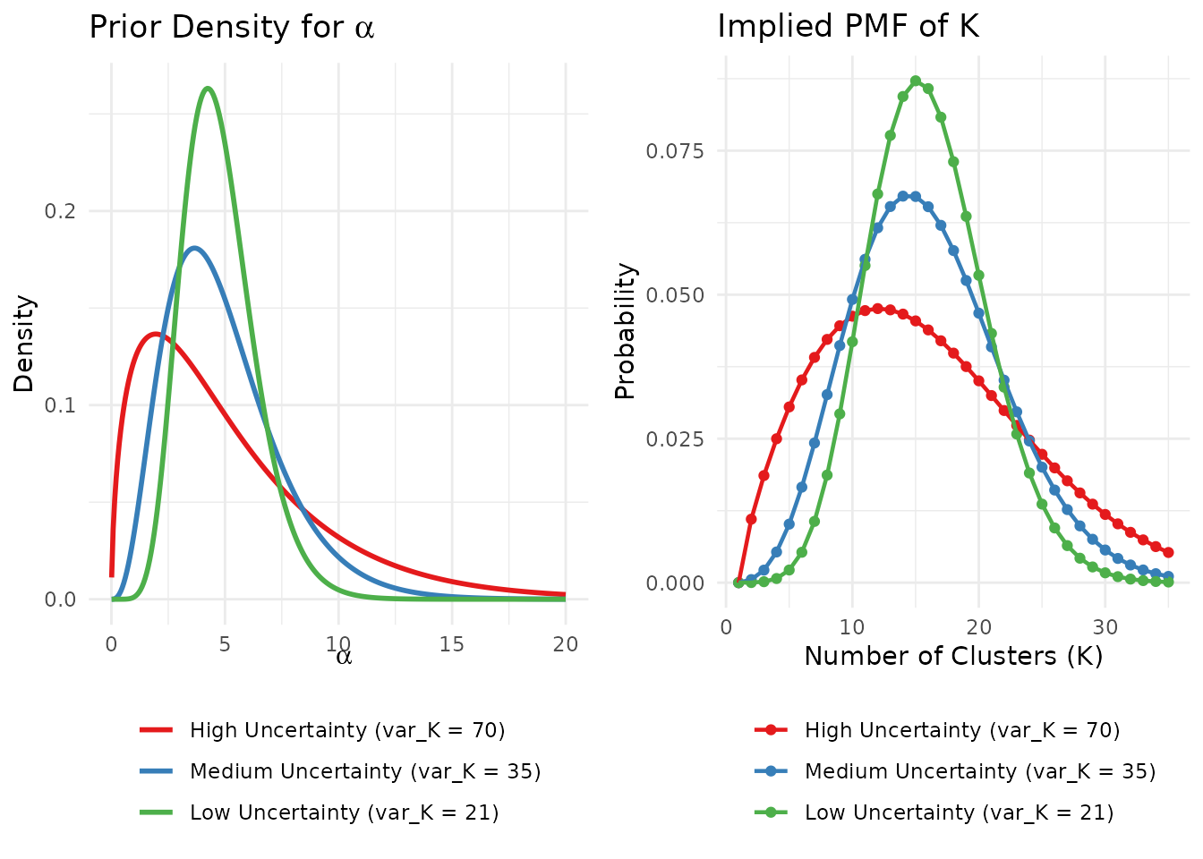

The same mean (μ_K = 15) with different levels of uncertainty leads to very different priors on α.

2. Eliciting the Mean: How Many Clusters?

The first step is determining $\mu_K$ , your expected number of clusters. This requires careful thought about your research context. Here are several strategies for arriving at a defensible value.

Understanding What $K_J$ Represents

Before eliciting $\mu_K$ , it is important to understand what $K_J$ represents. In the Dirichlet Process mixture model, $K_J$ denotes the number of occupied clusters among $J$ observations—not the total number of mixture components in the underlying model (which is infinite). As Lee et al. (2025) emphasize, $K_J$ functions more as an upper bound on the number of practically distinguishable subgroups rather than a precise count of “true” clusters.

This distinction has practical implications for elicitation:

Since $K_J$ tends to slightly overcount relative to the number of substantively meaningful groups, it is often reasonable to set $\mu_K$ somewhat generously—that is, slightly higher than your strict expectation for the number of “true” clusters.
A prior that allows for a few more clusters than you strictly expect provides flexibility for the data to reveal unexpected heterogeneity while still regularizing toward your domain knowledge.

Strategy 1: The Oracle Question

Imagine a trusted oracle who could reveal the true underlying pattern:

“If a reliable oracle showed you the true effect pattern across your 100 sites, approximately how many distinct groups would you see?”

This question bypasses abstract statistical thinking and focuses on substantive domain knowledge.

Strategy 2: Prior Research

Draw on previous studies in your field:

“In similar prior research, how many subtypes or subgroups have been identified?”

For example, in educational intervention research, previous meta-analyses might suggest that treatment effects typically cluster into 5-15 distinct patterns depending on the intervention type and population.

Strategy 3: Theoretical Mechanisms

Consider the underlying causal processes:

“How many distinct mechanisms or pathways do you theoretically expect to drive heterogeneity in your outcome?”

If your theory suggests multiple mechanisms (e.g., implementation fidelity, population characteristics, regional factors, and intervention dosage), you might set $\mu_K$ to accommodate their combinations.

Boundary Checks

Before proceeding, verify your $\mu_K$ satisfies basic constraints:

$\mu_K > 1$ : A single cluster is trivial and provides no insight into heterogeneity
$\mu_K < J$ : You cannot have more clusters than observations
Extreme values warrant careful consideration: $\mu_K$ close to $J$ implies you believe nearly every observation is unique

# Compare priors across different mu_K values
J <- 100
mu_K_values <- c(5, 10, 15, 25)

comparison_df <- data.frame(
  mu_K = mu_K_values,
  a = numeric(4),
  b = numeric(4),
  E_alpha = numeric(4),
  SD_alpha = numeric(4)
)

for (i in seq_along(mu_K_values)) {
  fit <- DPprior_fit(J, mu_K = mu_K_values[i], confidence = "low")
  comparison_df$a[i] <- fit$a
  comparison_df$b[i] <- fit$b
  comparison_df$E_alpha[i] <- fit$a / fit$b
  comparison_df$SD_alpha[i] <- sqrt(fit$a) / fit$b
}
#> Warning: HIGH DOMINANCE RISK: P(w1 > 0.5) = 60.6% exceeds 40%.
#>   This may indicate unintended prior behavior (RN-07).
#>   Consider using DPprior_dual() for weight-constrained elicitation.
#>   See ?DPprior_diagnostics for interpretation.

knitr::kable(
  comparison_df,
  col.names = c("Target μ_K", "a", "b", "E[α]", "SD(α)"),
  digits = 3,
  caption = "Gamma hyperparameters for different expected cluster counts 
  (J = 100, low confidence)"
)

Gamma hyperparameters for different expected cluster counts (J = 100, low confidence)
Target μ_K	a	b	E[α]	SD(α)
5	0.623	0.561	1.110	1.406
10	1.179	0.400	2.943	2.711
15	1.584	0.299	5.296	4.207
25	2.079	0.175	11.862	8.228

As the table shows, expecting more clusters leads to larger values of $E[\alpha]$ , reflecting the relationship between the concentration parameter and cluster formation in the Dirichlet Process.

3. Eliciting the Variance: How Certain Are You?

Once you have determined $\mu_K$ , you must express how certain you are about this value. The DPprior package offers three approaches, each suited to different contexts.

Method 1: Confidence Levels (Recommended for Most Users)

The simplest approach uses qualitative confidence levels that the package translates into appropriate variance specifications:

Level	VIF	Interpretation	Example var_K (μ_K = 15)
`"low"`	5.0	“I’m quite uncertain—this is a rough guess”	70
`"medium"`	2.5	“I have a reasonable sense but acknowledge uncertainty”	35
`"high"`	1.5	“I’m fairly confident based on strong prior evidence”	21

The VIF (Variance Inflation Factor) indicates how much larger the prior variance is relative to the baseline Poisson variance of $(\mu_K - 1)$ .

Recommendation: For most applied researchers seeking weakly informative priors, we recommend starting with confidence = "low". This provides regularization toward your expected cluster count while remaining flexible enough to let the data speak.

# Using confidence levels
fit_low    <- DPprior_fit(J = 100, mu_K = 15, confidence = "low")
fit_medium <- DPprior_fit(J = 100, mu_K = 15, confidence = "medium")
fit_high   <- DPprior_fit(J = 100, mu_K = 15, confidence = "high")

# What VIF values correspond to these levels?
cat("Low confidence VIF:   ", confidence_to_vif("low"), "\n")
#> Low confidence VIF:    5
cat("Medium confidence VIF:", confidence_to_vif("medium"), "\n")
#> Medium confidence VIF: 2.5
cat("High confidence VIF:  ", confidence_to_vif("high"), "\n")
#> High confidence VIF:   1.5

# Comparison table
confidence_comparison <- data.frame(
  Confidence = c("Low", "Medium", "High"),
  VIF = c(5.0, 2.5, 1.5),
  var_K = round(c(fit_low$target$var_K, fit_medium$target$var_K, 
                  fit_high$target$var_K), 2),
  a = round(c(fit_low$a, fit_medium$a, fit_high$a), 3),
  b = round(c(fit_low$b, fit_medium$b, fit_high$b), 3),
  CV_alpha = round(1/sqrt(c(fit_low$a, fit_medium$a, fit_high$a)), 3)
)

knitr::kable(
  confidence_comparison,
  col.names = c("Confidence", "VIF", "var_K", "a", "b", "CV(α)"),
  caption = "How confidence levels affect the elicited prior (J = 100, μ_K = 15)"
)

How confidence levels affect the elicited prior (J = 100, μ_K = 15)
Confidence	VIF	var_K	a	b	CV(α)
Low	5.0	70	1.584	0.299	0.794
Medium	2.5	35	3.916	0.797	0.505
High	1.5	21	8.993	1.885	0.333

Higher confidence leads to a smaller coefficient of variation (CV) for $\alpha$ , meaning the prior is more concentrated around its mean.

Method 2: Direct Variance Specification

For users who want precise control, you can specify $\text{Var}(K)$ directly:

# Specify variance directly
fit_direct <- DPprior_fit(J = 100, mu_K = 15, var_K = 50)
cat("Direct specification: var_K = 50\n")
#> Direct specification: var_K = 50
cat("  Gamma(a =", round(fit_direct$a, 3), ", b =", round(fit_direct$b, 3), ")\n")
#>   Gamma(a = 2.418 , b = 0.476 )
cat("  Achieved E[K] =", round(fit_direct$fit$mu_K, 4), "\n")
#>   Achieved E[K] = 15
cat("  Achieved Var(K) =", round(fit_direct$fit$var_K, 4), "\n")
#>   Achieved Var(K) = 50

Method 3: Quantile-Based Elicitation

A more intuitive approach for some researchers is to specify a credible interval for the number of clusters. For example:

“I believe there’s a 90% chance that the number of clusters falls between 8 and 25.”

Assuming a roughly symmetric distribution, this translates to a variance:

# Quantile-based elicitation
# 90% interval: [8, 25] with implied mean ~16.5
# Width = 17 = 2 × 1.645 × σ  →  σ ≈ 5.17  →  σ² ≈ 26.7

lower <- 8
upper <- 25
mu_K_quantile <- (lower + upper) / 2
sigma_K <- (upper - lower) / (2 * 1.645)  # 90% interval
var_K_quantile <- sigma_K^2

cat("From 90% interval [", lower, ", ", upper, "]:\n", sep = "")
#> From 90% interval [8, 25]:
cat("  Implied μ_K =", round(mu_K_quantile, 2), "\n")
#>   Implied μ_K = 16.5
cat("  Implied σ_K =", round(sigma_K, 2), "\n")
#>   Implied σ_K = 5.17
cat("  Implied var_K =", round(var_K_quantile, 2), "\n")
#>   Implied var_K = 26.7

fit_quantile <- DPprior_fit(J = 100, mu_K = mu_K_quantile, var_K = var_K_quantile)
cat("\nElicited prior: Gamma(", round(fit_quantile$a, 3), ", ", 
    round(fit_quantile$b, 3), ")\n", sep = "")
#> 
#> Elicited prior: Gamma(7.335, 1.322)

Method 4: VIF-Based Specification

If you think naturally in terms of relative variance, you can use the VIF directly:

# VIF-based specification
# "My uncertainty is about 5 times the Poisson baseline" (low confidence)
vif <- 5.0
var_K_vif <- vif_to_variance(mu_K = 15, vif = vif)

cat("VIF =", vif, "→ var_K =", var_K_vif, "\n")
#> VIF = 5 → var_K = 70

fit_vif <- DPprior_fit(J = 100, mu_K = 15, var_K = var_K_vif)
print(fit_vif)
#> DPprior Prior Elicitation Result
#> ============================================= 
#> 
#> Gamma Hyperprior: α ~ Gamma(a = 1.5843, b = 0.2992)
#>   E[α] = 5.296, SD[α] = 4.207
#> 
#> Target (J = 100):
#>   E[K_J]   = 15.00
#>   Var(K_J) = 70.00
#> 
#> Achieved:
#>   E[K_J] = 15.000000, Var(K_J) = 70.000000
#>   Residual = 5.86e-10
#> 
#> Method: A2-MN (6 iterations)
#> 
#> Dominance Risk: LOW ✓ (P(w₁>0.5) = 15%)

4. The Three Calibration Methods

The DPprior package offers three methods for calibrating the Gamma hyperparameters. Understanding when to use each method will help you make informed choices.

Method A1: Closed-Form Approximation

The A1 method provides an instantaneous, closed-form solution based on a Negative Binomial approximation to the $K$ distribution.

Pros:

Extremely fast (no iteration required)
Provides good accuracy for most practical cases
Useful for rapid exploration and initial calibration

Cons:

Slight approximation error, especially for small $J$ or extreme $\mu_K$
May project infeasible variance specifications to the boundary

fit_a1 <- DPprior_fit(J = 100, mu_K = 15, var_K = 70, method = "A1")

cat("Method A1 (Closed-Form Approximation)\n")
#> Method A1 (Closed-Form Approximation)
cat("  Gamma(a =", round(fit_a1$a, 4), ", b =", round(fit_a1$b, 4), ")\n")
#>   Gamma(a = 3.5 , b = 1.1513 )
cat("  Target:   E[K] =", fit_a1$target$mu_K, ", Var(K) =", fit_a1$target$var_K, "\n")
#>   Target:   E[K] = 15 , Var(K) = 70
cat("  Achieved: E[K] =", round(fit_a1$fit$mu_K, 4), 
    ", Var(K) =", round(fit_a1$fit$var_K, 4), "\n")
#>   Achieved: E[K] = 10.8439 , Var(K) = 23.0324
cat("  Residual:", format(fit_a1$fit$residual, scientific = TRUE), "\n")
#>   Residual: 4.715115e+01

Method A2-MN: Exact Moment Matching (Recommended)

The A2-MN method uses Newton iteration to find Gamma parameters that exactly match the target moments. This is the default and recommended method for most applications.

Pros:

Machine-precision accuracy
Guaranteed exact moment matching
Fast convergence (typically 5-10 iterations)

Cons:

Slightly slower than A1 (though still very fast)
Requires numerical iteration

fit_a2 <- DPprior_fit(J = 100, mu_K = 15, var_K = 70, method = "A2-MN")

cat("Method A2-MN (Exact Moment Matching)\n")
#> Method A2-MN (Exact Moment Matching)
cat("  Gamma(a =", round(fit_a2$a, 4), ", b =", round(fit_a2$b, 4), ")\n")
#>   Gamma(a = 1.5843 , b = 0.2992 )
cat("  Target:   E[K] =", fit_a2$target$mu_K, ", Var(K) =", fit_a2$target$var_K, "\n")
#>   Target:   E[K] = 15 , Var(K) = 70
cat("  Achieved: E[K] =", round(fit_a2$fit$mu_K, 6), 
    ", Var(K) =", round(fit_a2$fit$var_K, 6), "\n")
#>   Achieved: E[K] = 15 , Var(K) = 70
cat("  Residual:", format(fit_a2$fit$residual, scientific = TRUE), "\n")
#>   Residual: 5.855439e-10
cat("  Iterations:", fit_a2$iterations, "\n")
#>   Iterations: 6

Method A2-KL: KL Divergence Minimization

The A2-KL method minimizes the Kullback-Leibler divergence between a target PMF and the induced distribution of $K$ . This is useful when you have a specific target distribution in mind, not just moments.

Pros:

Matches the entire distribution shape, not just moments
Useful for custom target distributions
Faithful to the DORO (Discrepancy Optimization) philosophy (Dorazio, 2009)

Cons:

Requires specifying a target PMF
Computationally more intensive than moment matching

fit_kl <- DPprior_fit(J = 100, mu_K = 15, var_K = 70, method = "A2-KL")

cat("Method A2-KL (KL Divergence Minimization)\n")
#> Method A2-KL (KL Divergence Minimization)
cat("  Gamma(a =", round(fit_kl$a, 4), ", b =", round(fit_kl$b, 4), ")\n")
#>   Gamma(a = 1.767 , b = 0.3346 )
cat("  Target:   E[K] =", fit_kl$target$mu_K, ", Var(K) =", fit_kl$target$var_K, "\n")
#>   Target:   E[K] = 15 , Var(K) = 70
cat("  Achieved: E[K] =", round(fit_kl$fit$mu_K, 4), 
    ", Var(K) =", round(fit_kl$fit$var_K, 4), "\n")
#>   Achieved: E[K] = 15.0957 , Var(K) = 64.7345
cat("  Residual:", format(fit_kl$fit$residual, scientific = TRUE), "\n")
#>   Residual: 1.896688e-02

5. Comparing Methods

Let’s systematically compare the three methods across different scenarios:

compare_methods <- function(J, mu_K, var_K) {
  a1 <- DPprior_fit(J, mu_K, var_K, method = "A1")
  a2 <- DPprior_fit(J, mu_K, var_K, method = "A2-MN")
  kl <- DPprior_fit(J, mu_K, var_K, method = "A2-KL")
  
  data.frame(
    Method = c("A1", "A2-MN", "A2-KL"),
    a = round(c(a1$a, a2$a, kl$a), 4),
    b = round(c(a1$b, a2$b, kl$b), 4),
    `E[K]` = round(c(a1$fit$mu_K, a2$fit$mu_K, kl$fit$mu_K), 4),
    `Var(K)` = round(c(a1$fit$var_K, a2$fit$var_K, kl$fit$var_K), 4),
    Residual = format(c(a1$fit$residual, a2$fit$residual, kl$fit$residual), 
                      scientific = TRUE, digits = 2),
    check.names = FALSE
  )
}

# Standard case
cat("Scenario 1: J = 100, μ_K = 15, var_K = 70\n")
#> Scenario 1: J = 100, μ_K = 15, var_K = 70
knitr::kable(compare_methods(100, 15, 70))

Method	a	b	E[K]	Var(K)	Residual
A1	3.5000	1.1513	10.8439	23.0324	4.7e+01
A2-MN	1.5843	0.2992	15.0000	70.0000	5.9e-10
A2-KL	1.7670	0.3346	15.0957	64.7345	1.9e-02


# Large J
cat("\nScenario 2: J = 200, μ_K = 20, var_K = 95\n")
#> 
#> Scenario 2: J = 200, μ_K = 20, var_K = 95
knitr::kable(compare_methods(200, 20, 95))

Method	a	b	E[K]	Var(K)	Residual
A1	4.7500	1.3246	14.6529	34.4044	6.1e+01
A2-MN	2.4541	0.4283	20.0000	95.0000	2.7e-12
A2-KL	2.6502	0.4634	20.0459	89.5053	9.2e-03


# Smaller J
cat("\nScenario 3: J = 50, μ_K = 8, var_K = 35\n")
#> 
#> Scenario 3: J = 50, μ_K = 8, var_K = 35
knitr::kable(compare_methods(50, 8, 35))

Method	a	b	E[K]	Var(K)	Residual
A1	1.7500	0.9780	6.1497	12.4439	2.3e+01
A2-MN	0.7631	0.2433	8.0000	35.0000	7.1e-10
A2-KL	0.9298	0.2956	8.2100	31.4879	3.0e-02

Practical Recommendations

Based on the comparison:

For general use: Use A2-MN (the default). It provides exact moment matching with fast convergence.
For rapid exploration: Use A1 when you need instant results and can tolerate small approximation errors.
For distribution matching: Use A2-KL when you have a specific target distribution shape in mind.

6. Feasibility Constraints

Not all combinations of $(\mu_K, \sigma^2_K)$ are achievable with a Gamma hyperprior. Understanding these constraints helps you specify feasible targets.

Why Some Specifications Are Infeasible

The variance of $K$ under a Gamma hyperprior is bounded:

Lower bound: $\text{Var}(K) > \mu_K - 1$ (approximately). This is because the Negative Binomial proxy requires overdispersion relative to Poisson.
Upper bound: $\text{Var}(K) < (J-1)^2/4$ (approximately). This is a mathematical constraint on the variance of a bounded random variable.

How the Package Handles Infeasibility

# Example: Infeasible variance (too small)
cat("Attempting var_K = 10 (below feasible threshold for μ_K = 15):\n")
#> Attempting var_K = 10 (below feasible threshold for μ_K = 15):
fit_infeasible <- DPprior_fit(J = 100, mu_K = 15, var_K = 10, method = "A1")
#> Warning: A1 method: var_K=10.0000 < mu_K-1=14.0000 (infeasible for NegBin proxy).
#>   Projecting to feasible boundary: 14.000001
#> Warning: var_K <= mu_K - 1: projected to feasible boundary

cat("  Original var_K:", fit_infeasible$target$var_K, "\n")
#>   Original var_K: 10
cat("  Used var_K:", fit_infeasible$target$var_K_used, "\n")
#>   Used var_K: 14
cat("  (Projected to feasible boundary)\n")
#>   (Projected to feasible boundary)

The A1 method automatically projects infeasible specifications to the boundary of the feasible region. The A2-MN method attempts exact matching without projection, which may result in slower convergence or failure for truly infeasible targets.

7. A Complete Elicitation Workflow

Let’s walk through a complete, realistic example of prior elicitation.

Context

You are analyzing a multisite educational intervention study with 100 sites. Previous research on similar interventions has identified 8-20 distinct response patterns. Given the interpretation of $K_J$ as an upper bound on the number of distinguishable clusters (Lee et al., 2025), you decide to set your expectation generously at $\mu_K = 15$ .

# =============================================================================
# Step 1: Define the research context
# =============================================================================
J <- 100  # 100 sites
application_context <- "Multisite educational intervention study"

cat("Research Context:", application_context, "\n")
#> Research Context: Multisite educational intervention study
cat("Number of sites: J =", J, "\n\n")
#> Number of sites: J = 100

# =============================================================================
# Step 2: Determine μ_K based on domain knowledge
# =============================================================================
# Prior research suggests 8-20 response patterns
# Given K_J is an upper bound, we set μ_K generously at 15
mu_K <- 15

cat("Prior Knowledge:\n")
#> Prior Knowledge:
cat("  Previous studies found 8-20 response patterns\n")
#>   Previous studies found 8-20 response patterns
cat("  K_J serves as upper bound on distinguishable clusters\n")
#>   K_J serves as upper bound on distinguishable clusters
cat("  Selected μ_K =", mu_K, "(generous allowance for heterogeneity)\n\n")
#>   Selected μ_K = 15 (generous allowance for heterogeneity)

# =============================================================================
# Step 3: Determine uncertainty level
# =============================================================================
# For a weakly informative prior, we use low confidence
confidence <- "low"

cat("Uncertainty Assessment:\n")
#> Uncertainty Assessment:
cat("  Seeking weakly informative prior\n")
#>   Seeking weakly informative prior
cat("  Selected confidence:", confidence, "(recommended default)\n\n")
#>   Selected confidence: low (recommended default)

# =============================================================================
# Step 4: Fit the prior
# =============================================================================
fit <- DPprior_fit(
  J = J, 
  mu_K = mu_K, 
  confidence = confidence, 
  method = "A2-MN"
)

cat("Elicited Prior:\n")
#> Elicited Prior:
print(fit)
#> DPprior Prior Elicitation Result
#> ============================================= 
#> 
#> Gamma Hyperprior: α ~ Gamma(a = 1.5843, b = 0.2992)
#>   E[α] = 5.296, SD[α] = 4.207
#> 
#> Target (J = 100):
#>   E[K_J]   = 15.00
#>   Var(K_J) = 70.00
#>   (from confidence = 'low')
#> 
#> Achieved:
#>   E[K_J] = 15.000000, Var(K_J) = 70.000000
#>   Residual = 5.86e-10
#> 
#> Method: A2-MN (6 iterations)
#> 
#> Dominance Risk: LOW ✓ (P(w₁>0.5) = 15%)

Visualizing the Result

plot(fit)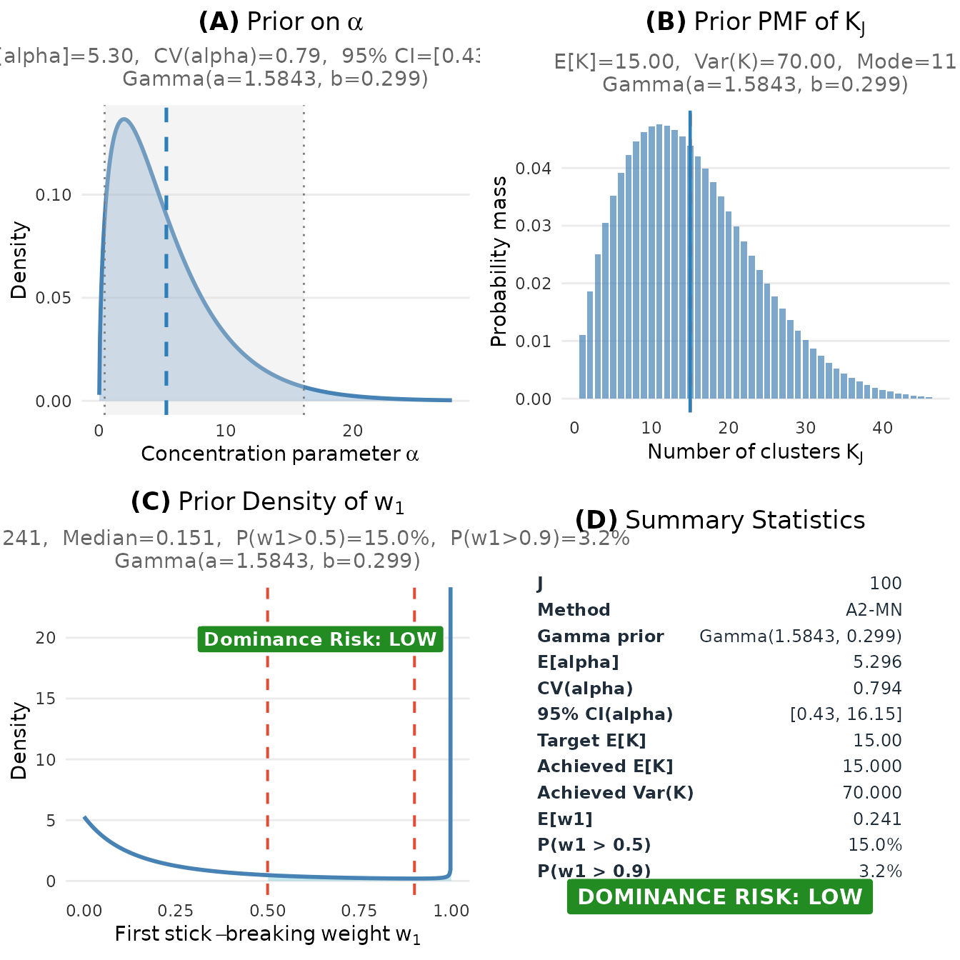

Complete visualization of the elicited prior for the educational intervention study.

#> TableGrob (2 x 2) "dpprior_dashboard": 4 grobs
#>   z     cells              name           grob
#> 1 1 (1-1,1-1) dpprior_dashboard gtable[layout]
#> 2 2 (2-2,1-1) dpprior_dashboard gtable[layout]
#> 3 3 (1-1,2-2) dpprior_dashboard gtable[layout]
#> 4 4 (2-2,2-2) dpprior_dashboard gtable[layout]

Extracting Results for Use in Bayesian Software

# Extract Gamma parameters for use in Stan, JAGS, etc.
cat("For Stan/JAGS:\n")
#> For Stan/JAGS:
cat("  alpha ~ gamma(", round(fit$a, 4), ", ", round(fit$b, 4), ");\n\n", sep = "")
#>   alpha ~ gamma(1.5843, 0.2992);

# Sample from the prior
n_samples <- 10000
alpha_samples <- rgamma(n_samples, shape = fit$a, rate = fit$b)

cat("Prior Summary (from", n_samples, "samples):\n")
#> Prior Summary (from 10000 samples):
cat("  E[α] =", round(mean(alpha_samples), 3), "\n")
#>   E[α] = 5.34
cat("  SD(α) =", round(sd(alpha_samples), 3), "\n")
#>   SD(α) = 4.294
cat("  95% CI: [", round(quantile(alpha_samples, 0.025), 3), ", ",
    round(quantile(alpha_samples, 0.975), 3), "]\n", sep = "")
#>   95% CI: [0.42, 16.565]

8. Sensitivity Analysis

A crucial part of responsible Bayesian analysis is understanding how your conclusions depend on your prior specifications. The DPprior package facilitates sensitivity analysis.

Sensitivity to μ_K

# How sensitive are the results to our choice of μ_K?
J <- 100
mu_K_grid <- c(8, 12, 15, 20)
sensitivity_mu <- lapply(mu_K_grid, function(mu) {
  DPprior_fit(J = J, mu_K = mu, confidence = "low")
})
#> Warning: HIGH DOMINANCE RISK: P(w1 > 0.5) = 40.4% exceeds 40%.
#>   This may indicate unintended prior behavior (RN-07).
#>   Consider using DPprior_dual() for weight-constrained elicitation.
#>   See ?DPprior_diagnostics for interpretation.

# Create comparison table
sensitivity_mu_df <- data.frame(
  `μ_K` = mu_K_grid,
  a = sapply(sensitivity_mu, function(x) round(x$a, 3)),
  b = sapply(sensitivity_mu, function(x) round(x$b, 3)),
  `E[α]` = sapply(sensitivity_mu, function(x) round(x$a / x$b, 3)),
  `P(w₁ > 0.5)` = sapply(sensitivity_mu, function(x) {
    round(prob_w1_exceeds(0.5, x$a, x$b), 3)
  }),
  check.names = FALSE
)

knitr::kable(
  sensitivity_mu_df,
  caption = "Sensitivity to μ_K (J = 100, low confidence)"
)

Sensitivity to μ_K (J = 100, low confidence)
μ_K	a	b	E[α]	P(w₁ > 0.5)
8	0.978	0.455	2.150	0.404
12	1.356	0.355	3.819	0.230
15	1.584	0.299	5.296	0.150
20	1.878	0.228	8.233	0.073


# Visualize with ggplot
alpha_grid <- seq(0.01, 25, length.out = 300)
sens_mu_df <- do.call(rbind, lapply(seq_along(sensitivity_mu), function(i) {
  fit <- sensitivity_mu[[i]]
  data.frame(
    alpha = alpha_grid,
    density = dgamma(alpha_grid, shape = fit$a, rate = fit$b),
    mu_K = paste0("μ_K = ", mu_K_grid[i])
  )
}))
sens_mu_df$mu_K <- factor(sens_mu_df$mu_K, 
                          levels = paste0("μ_K = ", mu_K_grid))

ggplot(sens_mu_df, aes(x = alpha, y = density, color = mu_K)) +
  geom_line(linewidth = 1) +
  scale_color_manual(values = palette_4) +
  labs(x = expression(alpha), y = "Density",
       title = expression("Prior Sensitivity to " * mu[K]),
       color = NULL) +
  theme_minimal() +
  theme(legend.position = "right")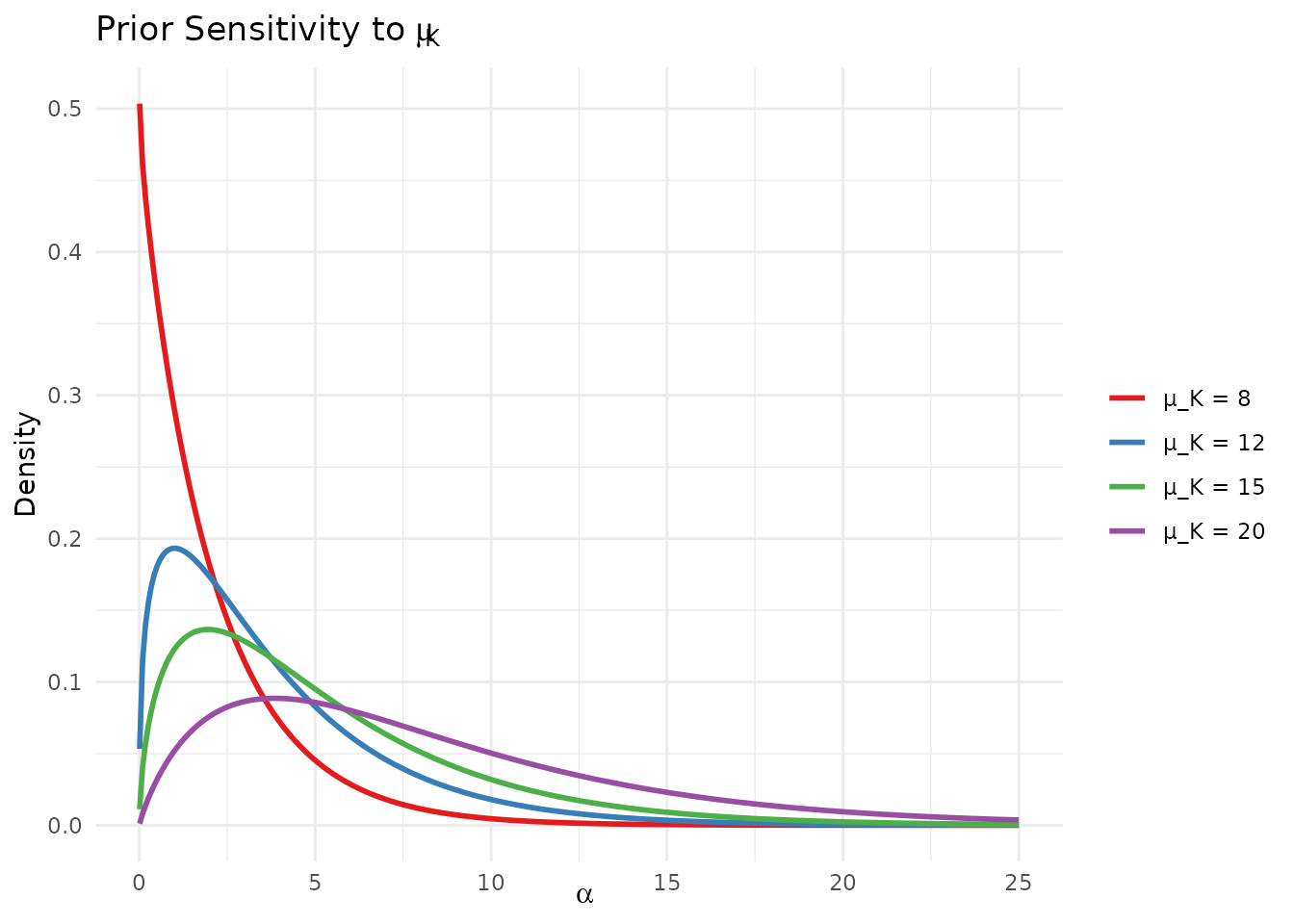

Sensitivity of the elicited prior to different expectations about the number of clusters.

Sensitivity to Confidence Level

# How sensitive are the results to our confidence level?
confidence_levels <- c("low", "medium", "high")
sensitivity_conf <- lapply(confidence_levels, function(conf) {
  DPprior_fit(J = 100, mu_K = 15, confidence = conf)
})

# Create comparison table
sensitivity_conf_df <- data.frame(
  Confidence = c("Low", "Medium", "High"),
  var_K = sapply(sensitivity_conf, function(x) round(x$target$var_K, 2)),
  a = sapply(sensitivity_conf, function(x) round(x$a, 3)),
  b = sapply(sensitivity_conf, function(x) round(x$b, 3)),
  `CV(α)` = sapply(sensitivity_conf, function(x) round(1/sqrt(x$a), 3)),
  `Median w₁` = sapply(sensitivity_conf, function(x) {
    round(quantile_w1(0.5, x$a, x$b), 3)
  }),
  check.names = FALSE
)

knitr::kable(
  sensitivity_conf_df,
  caption = "Sensitivity to confidence level (J = 100, μ_K = 15)"
)

Sensitivity to confidence level (J = 100, μ_K = 15)
Confidence	var_K	a	b	CV(α)	Median w₁
Low	70	1.584	0.299	0.794	0.151
Medium	35	3.916	0.797	0.505	0.143
High	21	8.993	1.885	0.333	0.140


# Visualize with ggplot
sens_conf_df <- do.call(rbind, lapply(seq_along(sensitivity_conf), function(i) {
  fit <- sensitivity_conf[[i]]
  data.frame(
    alpha = alpha_grid,
    density = dgamma(alpha_grid, shape = fit$a, rate = fit$b),
    Confidence = c("Low", "Medium", "High")[i]
  )
}))
sens_conf_df$Confidence <- factor(sens_conf_df$Confidence, 
                                  levels = c("Low", "Medium", "High"))

ggplot(sens_conf_df, aes(x = alpha, y = density, color = Confidence)) +
  geom_line(linewidth = 1) +
  scale_color_manual(values = palette_3) +
  labs(x = expression(alpha), y = "Density",
       title = "Prior Sensitivity to Confidence Level",
       color = NULL) +
  theme_minimal() +
  theme(legend.position = "right")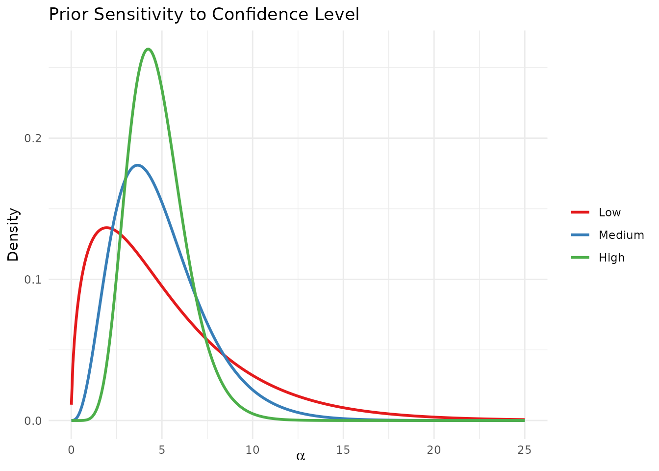

Sensitivity of the elicited prior to different confidence levels.

Comprehensive Sensitivity Analysis

For a thorough sensitivity analysis, you might want to explore a grid of specifications:

# Grid-based sensitivity analysis
mu_K_vals <- c(10, 15, 20)
conf_vals <- c("low", "medium", "high")

grid_results <- expand.grid(mu_K = mu_K_vals, confidence = conf_vals,
                            stringsAsFactors = FALSE)
grid_results$a <- NA
grid_results$b <- NA
grid_results$E_alpha <- NA

for (i in 1:nrow(grid_results)) {
  fit <- DPprior_fit(J = 100, 
                     mu_K = grid_results$mu_K[i], 
                     confidence = grid_results$confidence[i])
  grid_results$a[i] <- round(fit$a, 3)
  grid_results$b[i] <- round(fit$b, 3)
  grid_results$E_alpha[i] <- round(fit$a / fit$b, 3)
}

knitr::kable(
  grid_results,
  col.names = c("μ_K", "Confidence", "a", "b", "E[α]"),
  caption = "Comprehensive sensitivity analysis (J = 100)"
)

Comprehensive sensitivity analysis (J = 100)
μ_K	Confidence	a	b	E[α]
10	low	1.179	0.400	2.943
15	low	1.584	0.299	5.296
20	low	1.878	0.228	8.233
10	medium	2.992	1.100	2.720
15	medium	3.916	0.797	4.916
20	medium	4.556	0.596	7.643
10	high	7.185	2.728	2.634
15	high	8.993	1.885	4.772
20	high	10.129	1.365	7.422

Reporting Sensitivity Results

When reporting your analysis, we recommend:

Report your primary specification with clear justification
Show sensitivity results for at least ±3-5 units of $\mu_K$
Compare confidence levels to show how uncertainty affects inference
Discuss implications of any substantial differences in posterior conclusions

What’s Next?

This guide covered the fundamentals of cluster-count elicitation. For more advanced topics:

Dual-Anchor Framework: Learn to control both cluster count AND weight concentration simultaneously
Diagnostics: Verify your prior meets specifications and check for unintended consequences
Case Studies: See worked examples from education, medicine, and policy research
Mathematical Foundations: Understand the mathematical theory underlying the DPprior package

Summary

Step	Action	Key Function
1	Define context	`J <- ...`
2	Elicit expected clusters	`mu_K <- ...` (consider generous setting)
3	Express uncertainty	`confidence = "low"` (recommended default)
4	Choose method	`method = "A2-MN"` (default)
5	Fit prior	`fit <- DPprior_fit(J, mu_K, ...)`
6	Visualize	`plot(fit)`
7	Sensitivity analysis	Repeat with different specifications
8	Use in model	`alpha ~ gamma(fit$a, fit$b)`

References

Dorazio, R. M. (2009). On selecting a prior for the precision parameter of Dirichlet process mixture models. Journal of Statistical Planning and Inference, 139(9), 3384-3390. https://doi.org/10.1016/j.jspi.2009.03.009

Lee, J., Che, J., Rabe-Hesketh, S., Feller, A., & Miratrix, L. (2025). Improving the estimation of site-specific effects and their distribution in multisite trials. Journal of Educational and Behavioral Statistics, 50(5), 731–764. https://doi.org/10.3102/10769986241254286

For questions or feedback, please visit the GitHub repository.

JoonHo Lee

2026-01-01

Overview

1. The Elicitation Framework

The Two-Question Protocol

2. Eliciting the Mean: How Many Clusters?

Understanding What $K_J$ Represents

Strategy 1: The Oracle Question

Strategy 2: Prior Research

Strategy 3: Theoretical Mechanisms

Boundary Checks

3. Eliciting the Variance: How Certain Are You?

Method 1: Confidence Levels (Recommended for Most Users)

Method 2: Direct Variance Specification

Method 3: Quantile-Based Elicitation

Method 4: VIF-Based Specification

4. The Three Calibration Methods

Method A1: Closed-Form Approximation

Method A2-MN: Exact Moment Matching (Recommended)

Method A2-KL: KL Divergence Minimization

5. Comparing Methods

Practical Recommendations

6. Feasibility Constraints

Why Some Specifications Are Infeasible

How the Package Handles Infeasibility

7. A Complete Elicitation Workflow

Context

Visualizing the Result

Extracting Results for Use in Bayesian Software

8. Sensitivity Analysis

Sensitivity to μ_K

Sensitivity to Confidence Level

Comprehensive Sensitivity Analysis

Reporting Sensitivity Results

What’s Next?

Summary

References

The Applied Researcher's Guide to Cluster-Count Elicitation

JoonHo Lee

2026-01-01

Overview

1. The Elicitation Framework

The Two-Question Protocol

2. Eliciting the Mean: How Many Clusters?

Understanding What KJK_J Represents

Strategy 1: The Oracle Question

Strategy 2: Prior Research

Strategy 3: Theoretical Mechanisms

Boundary Checks

3. Eliciting the Variance: How Certain Are You?

Method 1: Confidence Levels (Recommended for Most Users)

Method 2: Direct Variance Specification

Method 3: Quantile-Based Elicitation

Method 4: VIF-Based Specification

4. The Three Calibration Methods

Method A1: Closed-Form Approximation

Method A2-MN: Exact Moment Matching (Recommended)

Method A2-KL: KL Divergence Minimization

5. Comparing Methods

Practical Recommendations

6. Feasibility Constraints

Why Some Specifications Are Infeasible

How the Package Handles Infeasibility

7. A Complete Elicitation Workflow

Context

Visualizing the Result

Extracting Results for Use in Bayesian Software

8. Sensitivity Analysis

Sensitivity to μ_K

Sensitivity to Confidence Level

Comprehensive Sensitivity Analysis

Reporting Sensitivity Results

What’s Next?

Summary

References

Understanding What $K_J$ Represents