Technical Deep Dive: Stirling Numbers and the Antoniak Distribution

JoonHo Lee

2026-01-01

Overview

This vignette provides a deep technical treatment of the computational machinery underlying the Antoniak distribution—the exact probability mass function (PMF) for the number of distinct clusters $K_J$ in a Dirichlet Process (DP) model. We focus specifically on unsigned Stirling numbers of the first kind and their numerically stable computation, which forms the core of the DPprior package’s reference computational layer.

This vignette is intended for statisticians and methodological researchers who want to understand the exact implementation details. We cover:

1. The combinatorial definition and properties of unsigned Stirling numbers
2. The computational challenge: why naive implementation fails
3. Log-space computation via the logsumexp trick
4. Computing the Antoniak PMF from Stirling numbers
5. Numerical stability analysis and implementation guards

Throughout, we distinguish between established results from the combinatorics and Bayesian nonparametrics literature and implementation contributions of this package.

1. Unsigned Stirling Numbers of the First Kind

1.1 Definition and Combinatorial Interpretation

The unsigned Stirling numbers of the first kind, denoted $|s(J, k)|$, count the number of permutations of $J$ elements that consist of exactly $k$ disjoint cycles.

Example. For $J = 3$ elements $\{1, 2, 3\}$, the permutations grouped by number of cycles are:

$k$	Permutations	Count $\|s(3,k)\|$
1	$(1\ 2\ 3), (1\ 3\ 2)$	2
2	$(1)(2\ 3), (2)(1\ 3), (3)(1\ 2)$	3
3	$(1)(2)(3)$	1

The total is $2 + 3 + 1 = 6 = 3!$, as expected since we’re partitioning all permutations.

Attribution. Stirling numbers have a rich history in combinatorics, dating back to James Stirling’s 1730 work Methodus Differentialis. The connection to the DP cluster distribution was established by Antoniak (1974).

1.2 Recurrence Relation

The unsigned Stirling numbers satisfy a fundamental recurrence:

$$|s(J, k)| = |s(J-1, k-1)| + (J-1) \cdot |s(J-1, k)|$$

Combinatorial interpretation: When adding element $J$ to a permutation of elements $\{1, \ldots, J-1\}$:

• Element $J$ can form a new cycle by itself: this accounts for $|s(J-1, k-1)|$ permutations (we need $k-1$ cycles in the first $J-1$ elements)
• Element $J$ can be inserted into any position within an existing cycle: there are $(J-1)$ positions to insert, and we need $k$ cycles already present, giving $(J-1) \cdot |s(J-1, k)|$

1.3 Boundary Conditions

The recurrence requires the following boundary conditions:

$$\begin{aligned} |s(0, 0)| &= 1 \quad \text{(empty permutation: one way to arrange nothing)} \\ |s(J, 0)| &= 0 \quad \text{for } J \geq 1 \text{ (no permutation has 0 cycles)} \\ |s(J, J)| &= 1 \quad \text{for all } J \text{ (only the identity has } J \text{ cycles)} \end{aligned}$$

1.4 Fundamental Identity

A crucial identity that serves as a computational verification is:

$$\sum_{k=1}^{J} |s(J, k)| = J!$$

This follows immediately from the fact that we’re partitioning all $J!$ permutations according to their cycle count.

# Compute log-Stirling numbers up to J = 15
logS <- compute_log_stirling(15)

# Verify known values
cat("Verification of known Stirling numbers:\n")
#> Verification of known Stirling numbers:
cat(sprintf("  |s(4, 2)| = %d (expected: 11)\n", round(exp(logS[5, 3]))))
#>   |s(4, 2)| = 11 (expected: 11)
cat(sprintf("  |s(5, 3)| = %d (expected: 35)\n", round(exp(logS[6, 4]))))
#>   |s(5, 3)| = 35 (expected: 35)
cat(sprintf("  |s(6, 3)| = %d (expected: 225)\n", round(exp(logS[7, 4]))))
#>   |s(6, 3)| = 225 (expected: 225)
cat(sprintf("  |s(10, 5)| = %d (expected: 269325)\n", round(exp(logS[11, 6]))))
#>   |s(10, 5)| = 269325 (expected: 269325)

# Verify row sum = J!
J_test <- 10
log_row_sum <- logsumexp_vec(logS[J_test + 1, 2:(J_test + 1)])
log_factorial <- sum(log(1:J_test))
cat(sprintf("\nRow sum identity for J = %d:\n", J_test))
#> 
#> Row sum identity for J = 10:
cat(sprintf("  sum_k |s(%d,k)| = %.0f\n", J_test, exp(log_row_sum)))
#>   sum_k |s(10,k)| = 3628800
cat(sprintf("  %d! = %.0f\n", J_test, exp(log_factorial)))
#>   10! = 3628800
cat(sprintf("  Relative error: %.2e\n", abs(exp(log_row_sum - log_factorial) - 1)))
#>   Relative error: 0.00e+00

2. The Computational Challenge

2.1 Explosive Growth of Stirling Numbers

The unsigned Stirling numbers grow extremely rapidly—faster than exponential. Consider some representative values:

Magnitude of Stirling numbers for various J

J	|s(J, 1)|	|s(J, ⌊J/2⌋)|	log₁₀(max |s(J,k)|)
10	3.6288e+05	2.69325e+05	5.56
20	1.2200e+17	1.40000e+13	17.09
50	6.0800e+62	1.05000e+52	62.78
100	9.3300e+156	3.70000e+130	156.97
200	NA	NA	373.02

For $J = 100$, the maximum Stirling number is approximately $10^{157}$, far exceeding the range of double-precision floating point ($\approx 10^{308}$ maximum, but with only 15-17 significant digits).

The key insight: Direct computation in the original scale is impossible for any practical $J$. We must work entirely in log-space.

2.2 Why Naive Log-Space Fails

One might think: “Just take logs of everything!” But consider the recurrence:

$$|s(J, k)| = |s(J-1, k-1)| + (J-1) \cdot |s(J-1, k)|$$

In log-space, this becomes:

$$\log|s(J, k)| = \log\left(e^{L_{J-1,k-1}} + (J-1) \cdot e^{L_{J-1,k}}\right)$$

where $L_{J,k} := \log|s(J,k)|$. The problem: we need to compute $\log(e^a + e^b)$ where $a$ and $b$ may be very large (causing overflow when exponentiating) or very different in magnitude (causing underflow when adding).

3. The logsumexp Trick

3.1 Mathematical Foundation

The logsumexp function computes $\log(e^a + e^b)$ in a numerically stable way using the identity:

$$\log(e^a + e^b) = \max(a, b) + \log\left(1 + e^{-|a-b|}\right)$$

Why this works:

1. The maximum is factored out, so we never exponentiate a large number
2. The argument to $\exp$ is always $\leq 0$, preventing overflow
3. We use log1p(x) = $\log(1 + x)$ for numerical stability near $x = 0$

3.2 Implementation and Verification

# Demonstrate numerical stability
cat("logsumexp numerical stability:\n")
#> logsumexp numerical stability:

# Case 1: Both arguments very large
a <- 1000
b <- 1000
result <- logsumexp(a, b)
expected <- 1000 + log(2)  # log(e^1000 + e^1000) = 1000 + log(2)
cat(sprintf("  logsumexp(1000, 1000) = %.6f (expected: %.6f)\n", result, expected))
#>   logsumexp(1000, 1000) = 1000.693147 (expected: 1000.693147)

# Case 2: Both arguments very negative
a <- -1000
b <- -1000
result <- logsumexp(a, b)
expected <- -1000 + log(2)
cat(sprintf("  logsumexp(-1000, -1000) = %.6f (expected: %.6f)\n", result, expected))
#>   logsumexp(-1000, -1000) = -999.306853 (expected: -999.306853)

# Case 3: Large difference in magnitude
a <- 1000
b <- -1000
result <- logsumexp(a, b)
cat(sprintf("  logsumexp(1000, -1000) = %.6f (essentially 1000)\n", result))
#>   logsumexp(1000, -1000) = 1000.000000 (essentially 1000)

# Case 4: Typical use case - log-sum of probabilities
log_p1 <- log(0.3)
log_p2 <- log(0.7)
result <- exp(logsumexp(log_p1, log_p2))
cat(sprintf("  exp(logsumexp(log(0.3), log(0.7))) = %.6f\n", result))
#>   exp(logsumexp(log(0.3), log(0.7))) = 1.000000

3.3 Vectorized Version

For computing $\log\sum_{i=1}^n e^{x_i}$, we use the vectorized extension:

$$\log\sum_{i=1}^n e^{x_i} = \max_i(x_i) + \log\sum_{i=1}^n e^{x_i - \max_i(x_i)}$$

# Demonstrate vectorized logsumexp
x <- c(100, 101, 102, 103)
result <- logsumexp_vec(x)
cat(sprintf("logsumexp_vec([100, 101, 102, 103]) = %.4f\n", result))
#> logsumexp_vec([100, 101, 102, 103]) = 103.4402
cat(sprintf("This equals: log(e^100 + e^101 + e^102 + e^103) ≈ log(e^103 * 1.52) = %.4f\n", 
            103 + log(1 + exp(-1) + exp(-2) + exp(-3))))
#> This equals: log(e^100 + e^101 + e^102 + e^103) ≈ log(e^103 * 1.52) = 103.4402

4. Computing the Log-Stirling Matrix

4.1 The Algorithm

The compute_log_stirling() function builds the complete lower-triangular matrix of log-Stirling numbers using the recursion:

$$L_{J,k} = \text{logsumexp}(L_{J-1,k-1}, \log(J-1) + L_{J-1,k})$$

Complexity: $O(J_{\max}^2)$ time and space.

# Compute the full log-Stirling matrix for J up to 50
J_max <- 50
logS <- compute_log_stirling(J_max)

cat(sprintf("Log-Stirling matrix dimensions: %d x %d\n", nrow(logS), ncol(logS)))
#> Log-Stirling matrix dimensions: 51 x 51
cat(sprintf("Memory usage: %.2f KB\n", object.size(logS) / 1024))
#> Memory usage: 20.53 KB

# Display a small section of the matrix (J = 1 to 10)
cat("\nlog|s(J, k)| for J = 1..10, k = 1..10:\n")
#> 
#> log|s(J, k)| for J = 1..10, k = 1..10:
small_section <- round(logS[2:11, 2:11], 2)
rownames(small_section) <- paste("J =", 1:10)
colnames(small_section) <- paste("k =", 1:10)
print(small_section)
#>        k = 1 k = 2 k = 3 k = 4 k = 5 k = 6 k = 7 k = 8 k = 9 k = 10
#> J = 1   0.00  -Inf  -Inf  -Inf  -Inf  -Inf  -Inf  -Inf  -Inf   -Inf
#> J = 2   0.00  0.00  -Inf  -Inf  -Inf  -Inf  -Inf  -Inf  -Inf   -Inf
#> J = 3   0.69  1.10  0.00  -Inf  -Inf  -Inf  -Inf  -Inf  -Inf   -Inf
#> J = 4   1.79  2.40  1.79  0.00  -Inf  -Inf  -Inf  -Inf  -Inf   -Inf
#> J = 5   3.18  3.91  3.56  2.30  0.00  -Inf  -Inf  -Inf  -Inf   -Inf
#> J = 6   4.79  5.61  5.42  4.44  2.71  0.00  -Inf  -Inf  -Inf   -Inf
#> J = 7   6.58  7.48  7.39  6.60  5.16  3.04  0.00  -Inf  -Inf   -Inf
#> J = 8   8.53  9.48  9.48  8.82  7.58  5.77  3.33  0.00  -Inf   -Inf
#> J = 9  10.60 11.60 11.68 11.12 10.02  8.42  6.30  3.58  0.00   -Inf
#> J = 10 12.80 13.84 13.97 13.49 12.50 11.06  9.15  6.77  3.81      0

4.2 Verification via Row Sums

We can verify the computation by checking that row sums equal $\log(J!)$:

# Verify row sum identity for multiple J values
cat("Verification of sum_k |s(J,k)| = J!:\n")
#> Verification of sum_k |s(J,k)| = J!:
cat(sprintf("%5s %15s %15s %12s\n", "J", "sum |s(J,k)|", "J!", "Rel. Error"))
#>     J    sum |s(J,k)|              J!   Rel. Error
cat(strrep("-", 48), "\n")
#> ------------------------------------------------

for (J in c(5, 10, 20, 30, 40, 50)) {
  log_row_sum <- logsumexp_vec(logS[J + 1, 2:(J + 1)])
  log_factorial <- sum(log(1:J))
  rel_error <- abs(exp(log_row_sum - log_factorial) - 1)
  
  # Display in scientific notation for large values
  cat(sprintf("%5d %15.4e %15.4e %12.2e\n", 
              J, exp(log_row_sum), exp(log_factorial), rel_error))
}
#>     5      1.2000e+02      1.2000e+02     0.00e+00
#>    10      3.6288e+06      3.6288e+06     0.00e+00
#>    20      2.4329e+18      2.4329e+18     7.11e-15
#>    30      2.6525e+32      2.6525e+32     1.42e-14
#>    40      8.1592e+47      8.1592e+47     1.42e-14
#>    50      3.0414e+64      3.0414e+64     2.84e-14

5. The Antoniak Distribution

5.1 Exact PMF of $K_J | \alpha$

The fundamental result connecting Stirling numbers to the DP cluster distribution is the Antoniak distribution (Antoniak, 1974):

$$\Pr(K_J = k | \alpha) = |s(J, k)| \cdot \frac{\alpha^k}{(\alpha)_J}, \quad k = 1, \ldots, J$$

where $(\alpha)_J = \alpha(\alpha+1)\cdots(\alpha+J-1) = \frac{\Gamma(\alpha+J)}{\Gamma(\alpha)}$ is the rising factorial (Pochhammer symbol).

Attribution. This formula was derived by Antoniak (1974) and is foundational to the Bayesian nonparametrics literature. It is restated in modern DP prior-elicitation work including Dorazio (2009), Murugiah and Sweeting (2012), and Vicentini and Jermyn (2025). Zito, Rigon, and Dunson (2024) present the general Gibbs-type form $\Pr(K_J = k) = V_{J,k} |s(J,k)|$.

5.2 Log-Space Computation

In log-space, the PMF becomes:

$$\log \Pr(K_J = k | \alpha) = \log|s(J, k)| + k \log\alpha - \log(\alpha)_J$$

where $\log(\alpha)_J = \log\Gamma(\alpha + J) - \log\Gamma(\alpha)$.

Normalization: The PMF is computed in log-space and then converted to probabilities via the softmax function, which ensures:

1. Numerical stability for extreme parameter values
2. Exact normalization to sum to 1

# Compute the Antoniak PMF for J = 50, alpha = 2
J <- 50
alpha <- 2

pmf <- pmf_K_given_alpha(J, alpha, logS)

# Verify normalization
cat(sprintf("PMF normalization check: sum(pmf) = %.10f\n", sum(pmf)))
#> PMF normalization check: sum(pmf) = 1.0000000000

# Summary statistics
k_vals <- 0:J
mean_K <- sum(k_vals * pmf)
var_K <- sum(k_vals^2 * pmf) - mean_K^2
mode_K <- which.max(pmf) - 1

cat(sprintf("\nDistribution of K_%d | α = %g:\n", J, alpha))
#> 
#> Distribution of K_50 | α = 2:
cat(sprintf("  E[K] = %.4f\n", mean_K))
#>   E[K] = 7.0376
cat(sprintf("  Var(K) = %.4f\n", var_K))
#>   Var(K) = 4.5356
cat(sprintf("  Mode(K) = %d\n", mode_K))
#>   Mode(K) = 7
cat(sprintf("  SD(K) = %.4f\n", sqrt(var_K)))
#>   SD(K) = 2.1297

5.3 Visualization

# Compute PMF for several alpha values
alpha_values <- c(0.5, 1, 2, 5, 10)
J <- 50

pmf_data <- do.call(rbind, lapply(alpha_values, function(a) {
  pmf <- pmf_K_given_alpha(J, a, logS)
  k_range <- 1:min(35, J)
  data.frame(
    k = k_range,
    pmf = pmf[k_range + 1],
    alpha = factor(paste0("α = ", a))
  )
}))

ggplot(pmf_data, aes(x = k, y = pmf, color = alpha)) +
  geom_line(linewidth = 1) +
  geom_point(size = 1.5) +
  scale_color_manual(values = c("#E41A1C", "#377EB8", "#4DAF4A", "#984EA3", "#FF7F00")) +
  labs(
    x = expression(k ~ "(number of clusters)"),
    y = expression(Pr(K[50] == k ~ "|" ~ alpha)),
    title = expression("Antoniak Distribution: " * Pr(K[J] == k ~ "|" ~ alpha)),
    subtitle = "J = 50 observations",
    color = "Concentration"
  ) +
  theme_minimal() +
  theme(
    legend.position = "right",
    plot.title = element_text(face = "bold", hjust = 0.5),
    plot.subtitle = element_text(hjust = 0.5)
  )

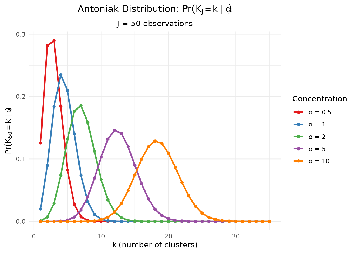
Antoniak PMF for various concentration parameters α with J = 50 observations.

5.4 Comparison with the Poisson-Binomial Representation

The Antoniak distribution can be alternatively derived from the Poisson-binomial representation (Theorem 1 in theory-overview):

$$K_J \stackrel{d}{=} \sum_{i=1}^{J} B_i, \quad B_i \sim \text{Bernoulli}\left(\frac{\alpha}{\alpha + i - 1}\right)$$

This provides an independent verification of our Stirling-based computation:

# Monte Carlo simulation using Poisson-Binomial representation
n_sim <- 100000
J <- 50
alpha <- 2

# Bernoulli success probabilities
p <- alpha / (alpha + (1:J) - 1)

# Simulate K_J
set.seed(123)
K_samples <- replicate(n_sim, sum(runif(J) < p))

# Compare distributions
k_range <- 1:20
pmf_stirling <- pmf_K_given_alpha(J, alpha, logS)[k_range + 1]
pmf_mc <- tabulate(K_samples, nbins = max(K_samples))[k_range] / n_sim

comparison_df <- data.frame(
  k = rep(k_range, 2),
  pmf = c(pmf_stirling, pmf_mc),
  Method = rep(c("Stirling (exact)", "Monte Carlo (n=100K)"), each = length(k_range))
)

ggplot(comparison_df, aes(x = k, y = pmf, color = Method, shape = Method)) +
  geom_point(size = 3, alpha = 0.8) +
  scale_color_manual(values = c("#E41A1C", "#377EB8")) +
  scale_shape_manual(values = c(16, 17)) +
  labs(
    x = expression(k),
    y = "Probability",
    title = expression("Verification: Stirling vs. Poisson-Binomial Monte Carlo"),
    subtitle = sprintf("J = %d, α = %g", J, alpha)
  ) +
  theme_minimal() +
  theme(
    legend.position = "bottom",
    plot.title = element_text(face = "bold", hjust = 0.5),
    plot.subtitle = element_text(hjust = 0.5)
  )
#> Warning: Removed 2 rows containing missing values or values outside the scale range
#> (`geom_point()`).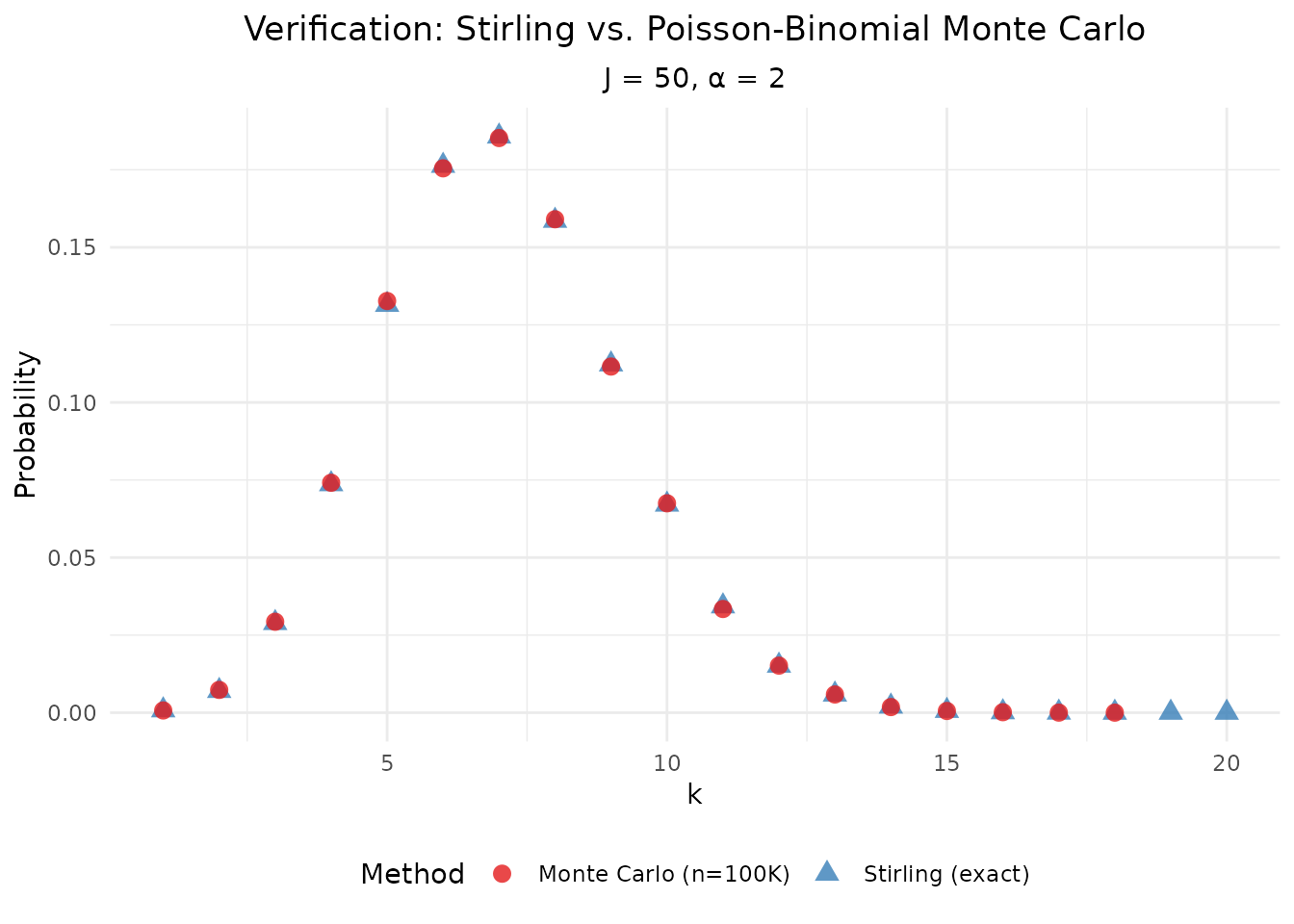

Verification: Stirling-based PMF vs. Monte Carlo from the Poisson-Binomial representation.

# Numerical comparison
max_diff <- max(abs(pmf_stirling - pmf_mc))
cat(sprintf("\nMaximum absolute difference between methods: %.2e\n", max_diff))
#> 
#> Maximum absolute difference between methods: NA

6. Numerical Stability Analysis

6.1 Critical Regions

The Antoniak PMF computation faces numerical challenges in extreme parameter regions:

Very small $\alpha$ (< 0.1): The distribution becomes highly concentrated at $K_J = 1$, with $\Pr(K_J = 1 | \alpha) \to 1$ as $\alpha \to 0$. This requires careful handling of probabilities very close to 1.

Very large $\alpha$ (> 50): The distribution shifts toward $K_J \approx J$, and the log-probabilities for small $k$ become extremely negative.

# Examine behavior at extreme alpha values
J <- 50
extreme_alphas <- c(0.01, 0.1, 1, 10, 50, 100)

cat("PMF stability at extreme α values (J = 50):\n")
#> PMF stability at extreme α values (J = 50):
cat(sprintf("%8s %12s %12s %12s %12s\n", 
            "α", "Pr(K=1)", "E[K]", "Mode(K)", "sum(pmf)"))
#>       α      Pr(K=1)         E[K]      Mode(K)     sum(pmf)
cat(strrep("-", 60), "\n")
#> ------------------------------------------------------------

for (a in extreme_alphas) {
  pmf <- pmf_K_given_alpha(J, a, logS)
  k_vals <- 0:J
  mean_K <- sum(k_vals * pmf)
  mode_K <- which.max(pmf) - 1
  sum_pmf <- sum(pmf)
  
  cat(sprintf("%8.2f %12.6f %12.2f %12d %12.10f\n", 
              a, pmf[2], mean_K, mode_K, sum_pmf))
}
#>     0.01     0.956274         1.04            1 1.0000000000
#>     0.10     0.643925         1.43            1 1.0000000000
#>     1.00     0.020000         4.50            4 1.0000000000
#>    10.00     0.000000        18.34           18 1.0000000000
#>    50.00     0.000000        34.91           35 1.0000000000
#>   100.00     0.000000        40.71           41 1.0000000000

6.2 Implementation Guards in DPprior

The DPprior package includes several defensive measures:

1. Log-space computation throughout: All intermediate calculations remain in log-space until the final softmax

2. Stable softmax: Uses the shifted exponential trick to prevent overflow: $p_i = \exp(x_i - \max_j x_j) / \sum_j \exp(x_j - \max_j x_j)$

3. Input validation: The assert_positive() and assert_valid_J() helpers catch invalid inputs early

4. Defensive renormalization: Final PMF vectors are explicitly normalized to sum to 1

6.3 Digamma Function Stability

The conditional moments of $K_J | \alpha$ involve the digamma function:

$$\mu_J(\alpha) = \alpha \cdot [\psi(\alpha + J) - \psi(\alpha)]$$

For very small $\alpha$, $\psi(\alpha) \to -\infty$, which can cause numerical issues. The package uses threshold-based switching to alternative formulations when needed:

# Compare digamma-based moments with PMF-based computation
J <- 50

alpha_test <- c(0.01, 0.1, 0.5, 1, 2, 5, 10)

cat("Moment computation consistency check:\n")
#> Moment computation consistency check:
cat(sprintf("%8s %12s %12s %12s\n", 
            "α", "E[K] (ψ)", "E[K] (PMF)", "Rel. Diff"))
#>       α    E[K] (ψ)   E[K] (PMF)    Rel. Diff
cat(strrep("-", 48), "\n")
#> ------------------------------------------------

for (a in alpha_test) {
  # Digamma-based computation
  mean_digamma <- mean_K_given_alpha(J, a)
  
  # PMF-based computation
  pmf <- pmf_K_given_alpha(J, a, logS)
  mean_pmf <- sum((0:J) * pmf)
  
  rel_diff <- abs(mean_digamma - mean_pmf) / mean_pmf
  
  cat(sprintf("%8.2f %12.6f %12.6f %12.2e\n", 
              a, mean_digamma, mean_pmf, rel_diff))
}
#>     0.01     1.044631     1.044631     8.50e-16
#>     0.10     1.432776     1.432776     1.08e-15
#>     0.50     2.937775     2.937775     2.12e-15
#>     1.00     4.499205     4.499205     1.38e-15
#>     2.00     7.037626     7.037626     2.90e-15
#>     5.00    12.460485    12.460485     2.14e-15
#>    10.00    18.342355    18.342355     2.13e-15

7. Computational Performance

7.1 Pre-computation Strategy

For typical use in prior elicitation (where $J$ is fixed for a given analysis), the log-Stirling matrix should be computed once and cached:

# Timing for log-Stirling matrix computation
J_values <- c(50, 100, 200, 300, 500)

cat("Log-Stirling matrix computation times:\n")
#> Log-Stirling matrix computation times:
cat(sprintf("%8s %15s %15s\n", "J_max", "Time (ms)", "Memory (KB)"))
#>    J_max       Time (ms)     Memory (KB)
cat(strrep("-", 40), "\n")
#> ----------------------------------------

for (J_max in J_values) {
  time_taken <- system.time({
    logS_temp <- compute_log_stirling(J_max)
  })["elapsed"] * 1000
  
  mem_kb <- object.size(logS_temp) / 1024
  
  cat(sprintf("%8d %15.2f %15.1f\n", J_max, time_taken, mem_kb))
}
#>       50            9.00            20.5
#>      100           39.00            79.9
#>      200          165.00           315.8
#>      300          363.00           708.0
#>      500         1000.00          1961.2

7.2 PMF Computation Timing

Once the Stirling matrix is cached, PMF computation is extremely fast:

# Pre-compute Stirling matrix
logS_300 <- compute_log_stirling(300)

# Time PMF computation for various J
cat("\nPMF computation times (with pre-computed Stirling matrix):\n")
#> 
#> PMF computation times (with pre-computed Stirling matrix):
cat(sprintf("%8s %8s %15s\n", "J", "α", "Time (μs)"))
#>        J       α      Time (μs)
cat(strrep("-", 35), "\n")
#> -----------------------------------

for (J in c(50, 100, 200, 300)) {
  for (alpha in c(1, 5)) {
    time_us <- mean(replicate(100, {
      t <- system.time(pmf_K_given_alpha(J, alpha, logS_300))["elapsed"]
    })) * 1e6
    
    cat(sprintf("%8d %8.1f %15.1f\n", J, alpha, time_us))
  }
}
#>       50      1.0            80.0
#>       50      5.0            30.0
#>      100      1.0            40.0
#>      100      5.0           160.0
#>      200      1.0           140.0
#>      200      5.0           130.0
#>      300      1.0           130.0
#>      300      5.0           110.0

8. Application: Effect of J on the Distribution

Understanding how the distribution of $K_J$ changes with sample size $J$ is crucial for prior elicitation. For fixed $\alpha$:

# Effect of J on K distribution
alpha <- 2
J_values <- c(20, 50, 100, 200)

logS_200 <- compute_log_stirling(200)

# Compute PMFs for different J
effect_data <- do.call(rbind, lapply(J_values, function(J) {
  pmf <- pmf_K_given_alpha(J, alpha, logS_200)
  k_max <- min(30, J)
  mean_K <- sum((0:J) * pmf)
  
  data.frame(
    k = 1:k_max,
    pmf = pmf[2:(k_max + 1)],
    J = factor(paste0("J = ", J, " (E[K] = ", round(mean_K, 1), ")"))
  )
}))

ggplot(effect_data, aes(x = k, y = pmf, color = J)) +
  geom_line(linewidth = 1) +
  geom_point(size = 1.5) +
  scale_color_manual(values = palette_main) +
  labs(
    x = expression(k ~ "(number of clusters)"),
    y = "Probability",
    title = expression("Effect of Sample Size on " * K[J] * " Distribution"),
    subtitle = expression("Fixed " * alpha * " = 2"),
    color = "Sample Size"
  ) +
  theme_minimal() +
  theme(
    legend.position = "right",
    plot.title = element_text(face = "bold", hjust = 0.5),
    plot.subtitle = element_text(hjust = 0.5)
  )

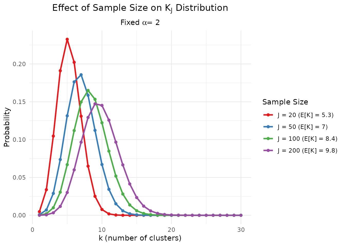
Effect of sample size J on the distribution of K for fixed α = 2.

Summary

This vignette has provided a detailed treatment of the computational machinery underlying the Antoniak distribution:

1. Unsigned Stirling numbers $|s(J,k)|$ count permutations with exactly $k$ cycles and satisfy a well-defined recurrence relation.

2. Numerical challenge: Direct computation overflows for $J > 20$; we must work entirely in log-space.

3. The logsumexp trick enables stable computation of $\log(e^a + e^b)$ for any values of $a$ and $b$.

4. The Antoniak distribution provides the exact PMF of $K_J | \alpha$ via Stirling numbers, computed stably in log-space.

5. DPprior implementation: Pre-computes and caches the log-Stirling matrix, enabling fast PMF evaluation for any $\alpha$.

The stable computation of the Antoniak PMF forms the foundation for the package’s exact moment-matching algorithms (A2) described in subsequent vignettes.

References

Antoniak, C. E. (1974). Mixtures of Dirichlet processes with applications to Bayesian nonparametric problems. The Annals of Statistics, 2(6), 1152-1174.

Arratia, R., Barbour, A. D., & Tavaré, S. (2003). Logarithmic Combinatorial Structures: A Probabilistic Approach. European Mathematical Society.

Dorazio, R. M. (2009). On selecting a prior for the precision parameter of Dirichlet process mixture models. Journal of Statistical Planning and Inference, 139(10), 3384-3390.

Murugiah, S., & Sweeting, T. J. (2012). Selecting the precision parameter prior in Dirichlet process mixture models. Journal of Statistical Planning and Inference, 142(7), 1947-1959.

Vicentini, C., & Jermyn, I. H. (2025). Prior selection for the precision parameter of Dirichlet process mixtures. arXiv:2502.00864.

Zito, A., Rigon, T., & Dunson, D. B. (2024). Bayesian nonparametric modeling of latent partitions via Stirling-gamma priors. arXiv:2306.02360.

Appendix: Key Function Reference

Function	Description
compute_log_stirling(J_max)	Pre-compute log-Stirling matrix for $J \leq J_{\max}$
get_log_stirling(J, k, logS)	Safe accessor with bounds checking
validate_stirling(logS)	Verify against known reference values
verify_stirling_row_sum(logS)	Verify $\sum_k \|s(J,k)\| = J!$ identity
logsumexp(a, b)	Numerically stable $\log(e^a + e^b)$
logsumexp_vec(x)	Vectorized log-sum-exp
softmax(x)	Numerically stable softmax
pmf_K_given_alpha(J, α, logS)	Antoniak PMF for $K_J \| \alpha$
log_pmf_K_given_alpha(J, α, logS)	Log-scale Antoniak PMF

---

For questions about this vignette or the DPprior package, please visit the GitHub repository.