Diagnosing Your Prior: Avoiding Unintended Consequences
JoonHo Lee
2026-05-07
Source:vignettes/diagnostics.Rmd
diagnostics.RmdOverview
When you elicit a Gamma hyperprior for based on your expectations about the number of clusters , you are implicitly specifying priors on many other quantities that you may not have consciously considered. These “unintended priors” can lead your posterior inference in unexpected directions, particularly in low-information settings where the data cannot overwhelm an inadvertently strong prior.
This vignette introduces the diagnostic tools in the DPprior package that help you verify your prior behaves as intended across all relevant dimensions. By the end, you will understand:
- Why diagnostics matter: the “unintended prior” problem
- The complete diagnostic suite available in DPprior
- How to interpret and weight distribution diagnostics
- The dominance warning system and how to respond to alerts
- How to use diagnostics to iteratively refine your prior
1. Why Diagnostics Matter
1.1 The Blind Spot in Prior Elicitation
The standard workflow for eliciting a DP prior focuses on cluster counts:
- You think about : “How many groups do I expect?”
- You think about : “How uncertain am I about that?”
- You call
DPprior_fit()and obtain
This is intuitive and principled. However, your elicited prior on determines not just , but also:
- The distribution of itself: mean, variance, and shape
- The cluster weight distribution: how mass is allocated across clusters
- The co-clustering probability: how likely two random observations share a cluster
- The dominance risk: probability that one cluster contains most of the data
These characteristics are implicit consequences of your choice. You may not have intended any particular behavior for these quantities, yet your prior assigns specific probabilities to them.
1.2 The Unintended Prior Problem
Vicentini & Jermyn (2025) demonstrated that matching a target distribution does not guarantee intuitive weight behavior. Consider a concrete example:
J <- 50
mu_K <- 5

# K-only calibration with moderate uncertainty
fit_K <- DPprior_fit(J = J, mu_K = mu_K, confidence = "low")
#> Warning: HIGH DOMINANCE RISK: P(w1 > 0.5) = 56.3% exceeds 40%.
#>   This may indicate unintended prior behavior (Lee, 2026).
#>   Consider using DPprior_dual() for weight-constrained elicitation.
#>   See ?DPprior_diagnostics for interpretation.

cat("K-only prior: Gamma(", round(fit_K$a, 3), ", ", round(fit_K$b, 3), ")\n", sep = "")
#> K-only prior: Gamma(0.518, 0.341)
cat("\nCluster count behavior:\n")
#>
#> Cluster count behavior:
cat("  E[K] =", round(exact_K_moments(J, fit_K$a, fit_K$b)$mean, 2), "\n")
#>   E[K] = 5
cat("  This matches our target of", mu_K, "clusters.\n")
#>   This matches our target of 5 clusters.

cat("\nBut what about weight behavior?\n")
#>
#> But what about weight behavior?
cat("  E[w₁] =", round(mean_w1(fit_K$a, fit_K$b), 3), "\n")
#>   E[w₁] = 0.585
cat("  P(w₁ > 0.3) =", round(prob_w1_exceeds(0.3, fit_K$a, fit_K$b), 3), "\n")
#>   P(w₁ > 0.3) = 0.69
cat("  P(w₁ > 0.5) =", round(prob_w1_exceeds(0.5, fit_K$a, fit_K$b), 3), "\n")
#>   P(w₁ > 0.5) = 0.563
cat("  P(w₁ > 0.9) =", round(prob_w1_exceeds(0.9, fit_K$a, fit_K$b), 3), "\n")
#>   P(w₁ > 0.9) = 0.346
The prior expects 5 clusters, but there is a substantial probability (nearly 50%) that a randomly selected observation belongs to a cluster containing more than half of all observations. Is this what you intended when you said “I expect 5 clusters”?
Most researchers, when they think “5 clusters,” imagine something like five roughly comparable groups—not a situation where one cluster might dominate the entire mixture.
1.3 Why This Matters in Practice
The unintended prior problem is especially consequential in low-information settings (Lee et al., 2025):
- Multisite trials with few sites: When is moderate (20–100), each site provides limited data
- Sparse clustering applications: When observations per cluster are small
- Exploratory analyses: When you don’t have strong prior data to inform expectations
In these settings, the posterior can remain close to the prior. If your prior inadvertently favors a single dominant cluster, your posterior may inherit this behavior even when the data suggest otherwise.
2. The Complete Diagnostic Suite
The DPprior package provides a comprehensive set of diagnostics that you can access in several ways.
2.1 Automatic Diagnostics During Fitting
The simplest approach is to enable diagnostics during the fitting process:
fit <- DPprior_fit(J = 50, mu_K = 5, var_K = 8, check_diagnostics = TRUE)
#> Warning: HIGH DOMINANCE RISK: P(w1 > 0.5) = 48.1% exceeds 40%.
#>   This may indicate unintended prior behavior (Lee, 2026).
#>   Consider using DPprior_dual() for weight-constrained elicitation.
#>   See ?DPprior_diagnostics for interpretation.
When check_diagnostics = TRUE, the function computes all
diagnostic quantities and stores them in the returned object.
2.2 Post-Hoc Diagnostic Computation
You can also compute diagnostics after fitting:
# Fit without diagnostics first
fit <- DPprior_fit(J = 50, mu_K = 5, var_K = 8)
#> Warning: HIGH DOMINANCE RISK: P(w1 > 0.5) = 48.1% exceeds 40%.
#>   This may indicate unintended prior behavior (Lee, 2026).
#>   Consider using DPprior_dual() for weight-constrained elicitation.
#>   See ?DPprior_diagnostics for interpretation.

# Then compute diagnostics
diag <- DPprior_diagnostics(fit)
print(diag)
#> DPprior Comprehensive Diagnostics
#> ============================================================
#>
#> Prior: alpha ~ Gamma(2.0361, 1.6051) for J = 50
#>
#> alpha Distribution:
#> ----------------------------------------
#>   E[alpha] = 1.269, CV(alpha) = 0.701, Median = 1.068
#>   90% CI: [0.230, 2.992]
#>
#> K_J Distribution:
#> ----------------------------------------
#>   E[K] = 5.00, SD(K) = 2.83, Mode = 3
#>   Median = 5, IQR = [3, 7]
#>
#> w1 Distribution (Size-Biased First Weight):
#> ----------------------------------------
#>   E[w1] = 0.501, Median = 0.478
#>   P(w1 > 0.5) = 48.1% (dominance risk: HIGH)
#>   P(w1 > 0.9) = 16.3%
#>
#> Co-Clustering (rho = sum w_h^2):
#> ----------------------------------------
#>   E[rho] = 0.501 (High prior co-clustering: most unit pairs expected in same cluster)
#>
#> WARNINGS:
#> ----------------------------------------
#>   * HIGH DOMINANCE RISK: P(w1 > 0.5) = 48.1% exceeds 40%
#>   * NEAR-DEGENERATE RISK: P(w1 > 0.9) = 16.3% exceeds 15%
#>
#>   Consider using DPprior_dual() for weight-constrained elicitation.
2.3 Overview of Diagnostic Components
The diagnostic object contains several components:
| Component | Description |
|---|---|
alpha |
Properties of the prior (mean, SD, CV, quantiles) |
K |
Properties of the marginal (mean, variance, mode, PMF) |
weights |
First stick-breaking weight distribution (mean, median, tail probabilities) |
coclustering |
Co-clustering probability summary |
warnings |
Character vector of any diagnostic warnings |
Let us examine each component in detail.
3. Alpha Distribution Diagnostics
The first set of diagnostics concerns the concentration parameter itself. Since , we can compute all moments analytically.
3.1 Accessing Alpha Diagnostics
fit <- DPprior_fit(J = 50, mu_K = 5, var_K = 8)
#> Warning: HIGH DOMINANCE RISK: P(w1 > 0.5) = 48.1% exceeds 40%.
#>   This may indicate unintended prior behavior (Lee, 2026).
#>   Consider using DPprior_dual() for weight-constrained elicitation.
#>   See ?DPprior_diagnostics for interpretation.
diag <- DPprior_diagnostics(fit)

cat("Alpha distribution summary:\n")
#> Alpha distribution summary:
cat("  Mean:     E[α] =", round(diag$alpha$mean, 4), "\n")
#>   Mean:     E[α] = 1.2686
cat("  SD:       SD(α) =", round(diag$alpha$sd, 4), "\n")
#>   SD:       SD(α) = 0.889
cat("  CV:       CV(α) =", round(diag$alpha$cv, 4), "\n")
#>   CV:       CV(α) = 0.7008
cat("\nQuantiles:\n")
#>
#> Quantiles:
cat("   5th percentile:", round(diag$alpha$quantiles["q5"], 4), "\n")
#>    5th percentile: 0.2305
cat("  25th percentile:", round(diag$alpha$quantiles["q25"], 4), "\n")
#>   25th percentile: 0.6155
cat("  50th percentile:", round(diag$alpha$quantiles["q50"], 4), "\n")
#>   50th percentile: 1.068
cat("  75th percentile:", round(diag$alpha$quantiles["q75"], 4), "\n")
#>   75th percentile: 1.7058
cat("  95th percentile:", round(diag$alpha$quantiles["q95"], 4), "\n")
#>   95th percentile: 2.992
3.2 Interpreting the Coefficient of Variation
The coefficient of variation (CV) of is particularly informative:
| CV Range | Interpretation |
|---|---|
| CV < 0.3 | Highly informative: You are quite certain about |
| 0.3 ≤ CV < 0.5 | Moderately informative: Reasonable uncertainty |
| 0.5 ≤ CV < 1.0 | Weakly informative: Substantial uncertainty about |
| CV ≥ 1.0 | Highly diffuse: Very uncertain about |
For a Gamma distribution, , so the CV depends only on the shape parameter .
# Compare different CV levels
a_values <- c(0.5, 1, 2, 4, 10)
cv_values <- 1 / sqrt(a_values)

alpha_grid <- seq(0.01, 8, length.out = 300)
cv_df <- do.call(rbind, lapply(seq_along(a_values), function(i) {
  a <- a_values[i]
  # Use b = a so E[alpha] = 1 for all
  b <- a
  data.frame(
    alpha = alpha_grid,
    density = dgamma(alpha_grid, shape = a, rate = b),
    CV = sprintf("CV = %.2f (a = %.1f)", cv_values[i], a)
  )
}))
cv_df$CV <- factor(cv_df$CV, levels = unique(cv_df$CV))

ggplot(cv_df, aes(x = alpha, y = density, color = CV)) +
  geom_line(linewidth = 1) +
  scale_color_viridis_d(option = "plasma", end = 0.85) +
  labs(
    x = expression(alpha),
    y = "Density",
    title = "Prior Informativeness Controlled by Shape Parameter",
    subtitle = "All priors have E[α] = 1; higher a means lower CV (more informative)"
  ) +
  theme_minimal() +
  theme(legend.position = "right")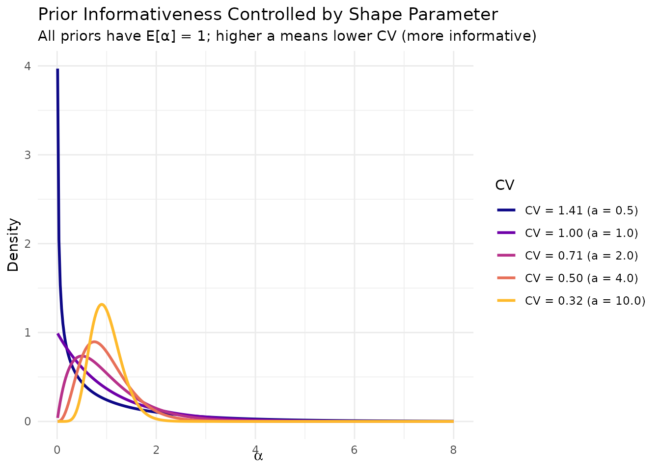
Different levels of informativeness in the α prior, controlled by the shape parameter a.
4. Weight Distribution Diagnostics
The weight diagnostics are crucial for detecting unintended prior behavior. The DPprior package provides comprehensive diagnostics for the first stick-breaking weight .
4.1 Understanding
Recall from the Dual-Anchor vignette that under Sethuraman’s stick-breaking representation:
The quantity has a natural interpretation: it is the proportion of the cluster containing a randomly selected observation. If is high, a random observation is likely to belong to a cluster containing more than half of all observations.
4.2 Accessing Weight Diagnostics
cat("Weight distribution summary:\n")
#> Weight distribution summary:
cat("  E[w₁] =", round(diag$weights$mean, 4), "\n")
#>   E[w₁] = 0.5014
cat("  Median(w₁) =", round(diag$weights$median, 4), "\n")
#>   Median(w₁) = 0.4784

cat("\nDominance tail probabilities:\n")
#>
#> Dominance tail probabilities:
cat("  P(w₁ > 0.3) =", round(diag$weights$prob_exceeds["prob_gt_0.3"], 4), "\n")
#>   P(w₁ > 0.3) = NA
cat("  P(w₁ > 0.5) =", round(diag$weights$prob_exceeds["prob_gt_0.5"], 4), "\n")
#>   P(w₁ > 0.5) = 0.4815
cat("  P(w₁ > 0.7) =", round(diag$weights$prob_exceeds["prob_gt_0.7"], 4), "\n")
#>   P(w₁ > 0.7) = NA
cat("  P(w₁ > 0.9) =", round(diag$weights$prob_exceeds["prob_gt_0.9"], 4), "\n")
#>   P(w₁ > 0.9) = 0.1634

cat("\nDominance risk level:", toupper(diag$weights$dominance_risk), "\n")
#>
#> Dominance risk level: HIGH
4.3 Closed-Form Calculations
All diagnostics are computed using closed-form expressions (derived in Lee, 2026, following Vicentini & Jermyn, 2025):
CDF:
Quantile function:
Tail probability (dominance risk):
You can access these functions directly:
a <- fit$a
b <- fit$b

# Direct computation of tail probabilities
cat("Direct computation of P(w₁ > t):\n")
#> Direct computation of P(w₁ > t):
for (t in c(0.3, 0.5, 0.7, 0.9)) {
  p <- prob_w1_exceeds(t, a, b)
  cat(sprintf("  P(w₁ > %.1f) = %.4f\n", t, p))
}
#>   P(w₁ > 0.3) = 0.6646
#>   P(w₁ > 0.5) = 0.4815
#>   P(w₁ > 0.7) = 0.3200
#>   P(w₁ > 0.9) = 0.1634

# Quantiles
cat("\nQuantiles of w₁ distribution:\n")
#>
#> Quantiles of w₁ distribution:
for (q in c(0.25, 0.5, 0.75, 0.95)) {
  x <- quantile_w1(q, a, b)
  cat(sprintf("  %d%% quantile: %.4f\n", round(100*q), x))
}
#>   25% quantile: 0.2162
#>   50% quantile: 0.4784
#>   75% quantile: 0.7911
#>   95% quantile: 0.9954
5. The Dominance Warning System
The DPprior package includes an automatic warning system to alert you when your prior implies a high probability of cluster dominance.
5.1 Dominance Risk Levels
The dominance risk is categorized into three levels based on :
| Risk Level | Criterion | Interpretation |
|---|---|---|
| LOW | Cluster balance is likely; weights spread across multiple clusters | |
| MODERATE | Some chance of dominance; consider your tolerance | |
| HIGH | Substantial dominance risk; action recommended |
5.2 Enabling Dominance Warnings
You can enable automatic warnings during fitting:
# A prior with high dominance risk
fit_risky <- DPprior_fit(J = 50, mu_K = 2, var_K = 2, warn_dominance = TRUE)
#> Warning: HIGH DOMINANCE RISK: P(w1 > 0.5) = 85.1% exceeds 40%.
#>   This may indicate unintended prior behavior (Lee, 2026).
#>   Consider using DPprior_dual() for weight-constrained elicitation.
#>   See ?DPprior_diagnostics for interpretation.
When warn_dominance = TRUE, the function will issue a
warning if the dominance risk is HIGH.
5.3 Checking Dominance Risk Manually
You can also check the dominance risk from the diagnostic object:
diag_risky <- DPprior_diagnostics(fit_risky)

cat("Dominance risk assessment:\n")
#> Dominance risk assessment:
cat("  Risk level:", toupper(diag_risky$weights$dominance_risk), "\n")
#>   Risk level: HIGH
cat("  P(w₁ > 0.5) =", round(diag_risky$weights$prob_exceeds["prob_gt_0.5"], 4), "\n")
#>   P(w₁ > 0.5) = 0.8511
5.4 What High Dominance Means
A HIGH dominance risk means your prior places substantial probability on scenarios where the size-biased first stick-breaking cluster mass exceeds one half. This may or may not be appropriate depending on your application:
When high dominance might be appropriate:
- You genuinely expect most data to fall into one dominant group
- You are modeling rare events where most observations are “baseline”
- You have strong prior evidence of an unbalanced partition
When high dominance is likely unintended:
- You expect roughly equal-sized clusters
- You think “ clusters” should mean roughly balanced groups
- You are doing exploratory clustering without strong prior expectations
5.5 Responding to High Dominance Warnings
If you receive a high dominance warning and it is unintended, you have several options:
- Increase : Expecting more clusters typically reduces dominance risk
- Decrease : More certainty about cluster count can help
- Use dual-anchor elicitation: Directly constrain weight behavior
We will demonstrate option 3 in Section 7.
6. Visualizing Diagnostics
The DPprior package provides several visualization functions for understanding your prior.
6.1 The Complete Dashboard
The plot() method for a DPprior_fit object
creates a comprehensive four-panel dashboard:
fit <- DPprior_fit(J = 50, mu_K = 5, var_K = 8)
#> Warning: HIGH DOMINANCE RISK: P(w1 > 0.5) = 48.1% exceeds 40%.
#>   This may indicate unintended prior behavior (Lee, 2026).
#>   Consider using DPprior_dual() for weight-constrained elicitation.
#>   See ?DPprior_diagnostics for interpretation.
plot(fit)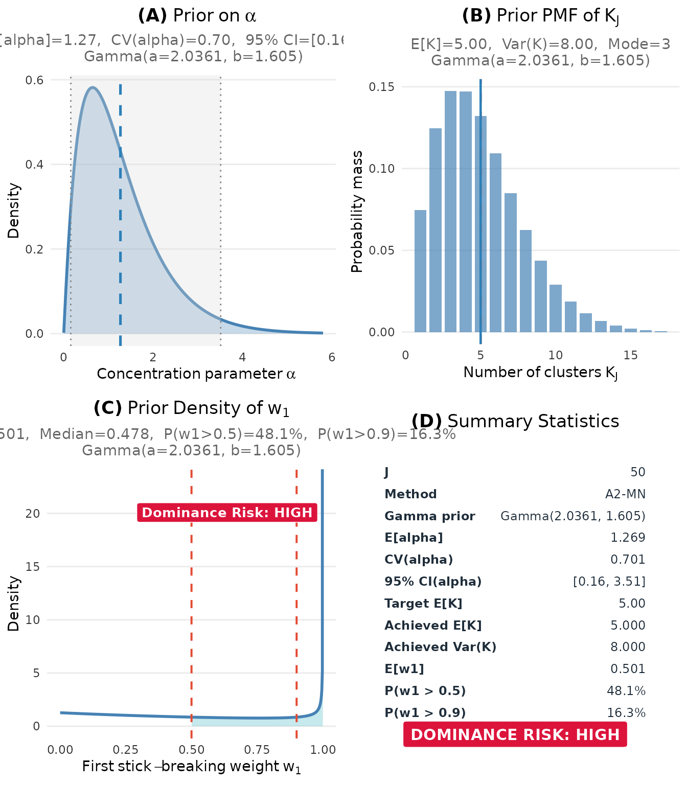
Complete diagnostic dashboard showing all key prior characteristics.
#> TableGrob (2 x 2) "dpprior_dashboard": 4 grobs
#>   z     cells              name           grob
#> 1 1 (1-1,1-1) dpprior_dashboard gtable[layout]
#> 2 2 (2-2,1-1) dpprior_dashboard gtable[layout]
#> 3 3 (1-1,2-2) dpprior_dashboard gtable[layout]
#> 4 4 (2-2,2-2) dpprior_dashboard gtable[layout]
6.2 Individual Diagnostic Plots
For more focused analysis, you can create individual plots:
# Alpha prior density
plot_alpha_prior(fit)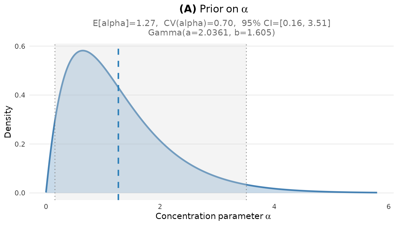
Prior density for the concentration parameter alpha.
# K marginal PMF
plot_K_prior(fit)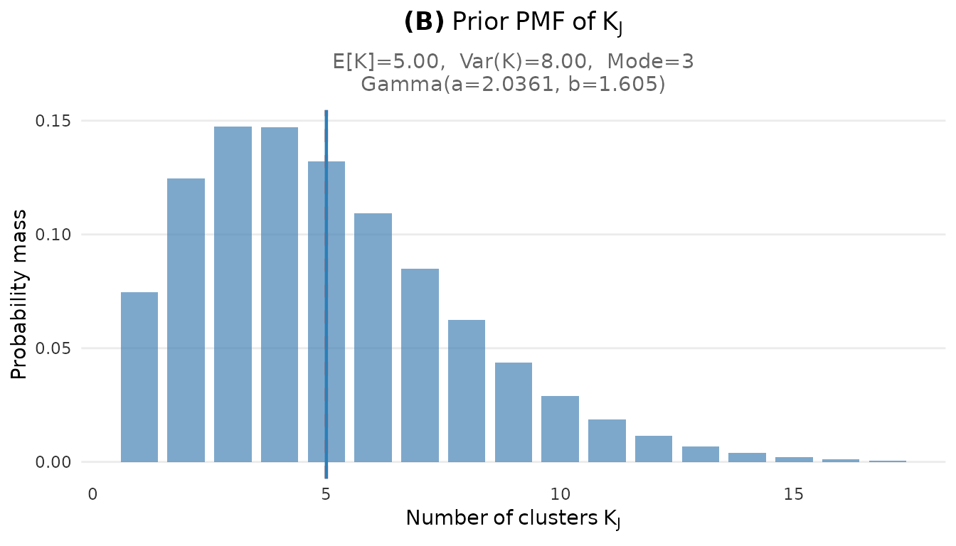
Marginal PMF of the number of clusters K.
# w1 distribution with dominance thresholds
plot_w1_prior(fit)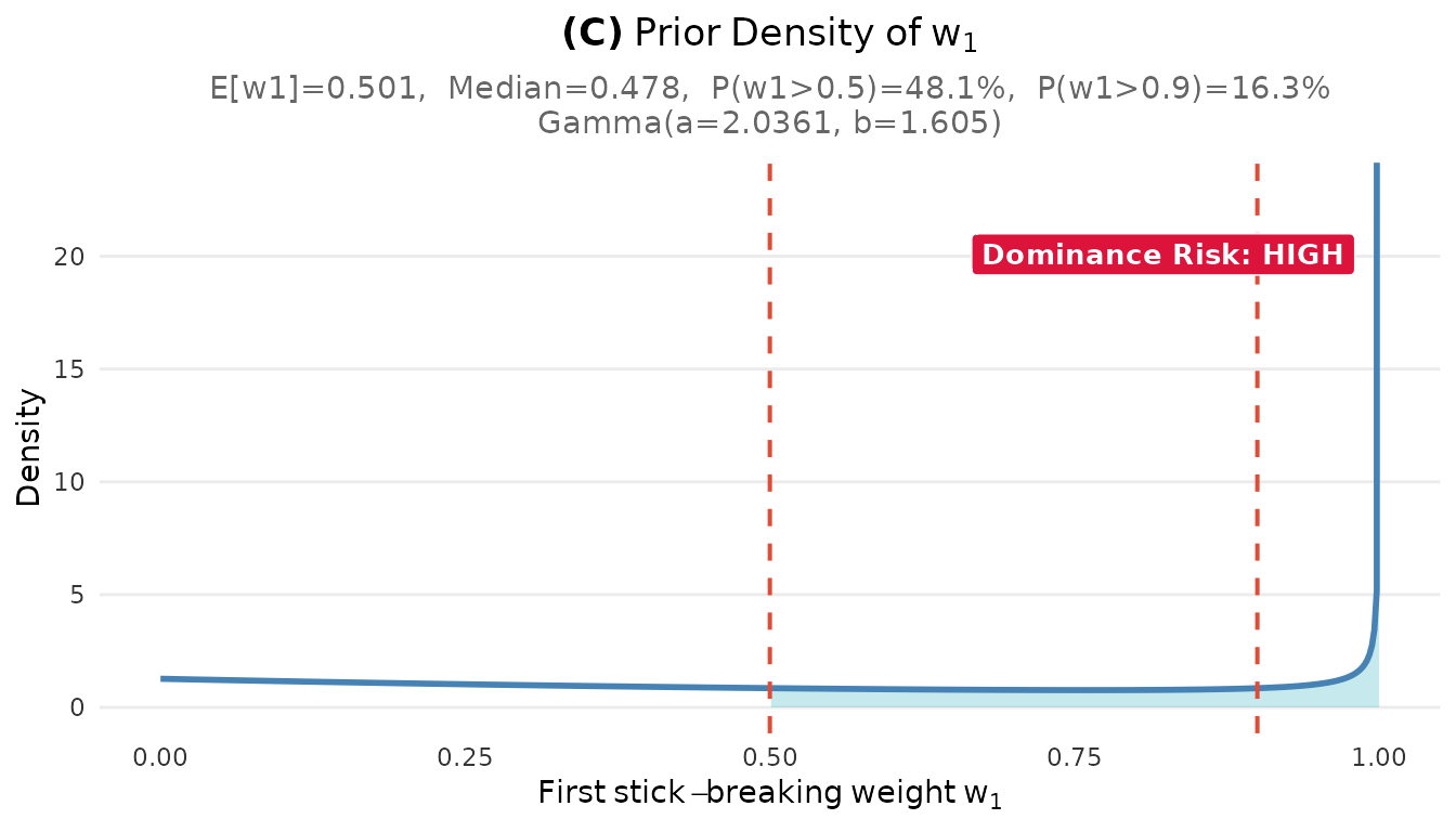
Distribution of the first stick-breaking weight w1.
6.3 Comparing Multiple Priors
When considering different prior specifications, you can visualize them side by side:
fits <- list(
  "Low uncertainty (var_K = 6)" = DPprior_fit(J = 50, mu_K = 5, var_K = 6),
  "Medium uncertainty (var_K = 10)" = DPprior_fit(J = 50, mu_K = 5, var_K = 10),
  "High uncertainty (var_K = 20)" = DPprior_fit(J = 50, mu_K = 5, var_K = 20)
)
#> Warning: HIGH DOMINANCE RISK: P(w1 > 0.5) = 46.5% exceeds 40%.
#>   This may indicate unintended prior behavior (Lee, 2026).
#>   Consider using DPprior_dual() for weight-constrained elicitation.
#>   See ?DPprior_diagnostics for interpretation.
#> Warning: HIGH DOMINANCE RISK: P(w1 > 0.5) = 49.7% exceeds 40%.
#>   This may indicate unintended prior behavior (Lee, 2026).
#>   Consider using DPprior_dual() for weight-constrained elicitation.
#>   See ?DPprior_diagnostics for interpretation.
#> Warning: HIGH DOMINANCE RISK: P(w1 > 0.5) = 56.3% exceeds 40%.
#>   This may indicate unintended prior behavior (Lee, 2026).
#>   Consider using DPprior_dual() for weight-constrained elicitation.
#>   See ?DPprior_diagnostics for interpretation.

# Compute log Stirling numbers for efficiency
logS <- compute_log_stirling(50)

# Build comparison data
k_df <- do.call(rbind, lapply(names(fits), function(nm) {
  fit <- fits[[nm]]
  pmf <- pmf_K_marginal(50, fit$a, fit$b, logS = logS)
  data.frame(
    K = seq_along(pmf) - 1,  # pmf_K_marginal returns k=0,...,J
    probability = pmf,
    Prior = nm
  )
}))
k_df <- k_df[k_df$K >= 1, ]  # Remove k=0
k_df$Prior <- factor(k_df$Prior, levels = names(fits))

# Plot
ggplot(k_df[k_df$K <= 20, ], aes(x = K, y = probability, color = Prior)) +
  geom_point(size = 2) +
  geom_line(linewidth = 0.8) +
  scale_color_manual(values = palette_3) +
  labs(
    x = expression(Number~of~clusters~K[J]),
    y = "Probability",
    title = "Prior PMF of K Under Different Variance Assumptions",
    subtitle = "All priors have μ_K = 5; higher variance spreads the distribution"
  ) +
  theme_minimal() +
  theme(legend.position = "bottom", legend.title = element_blank())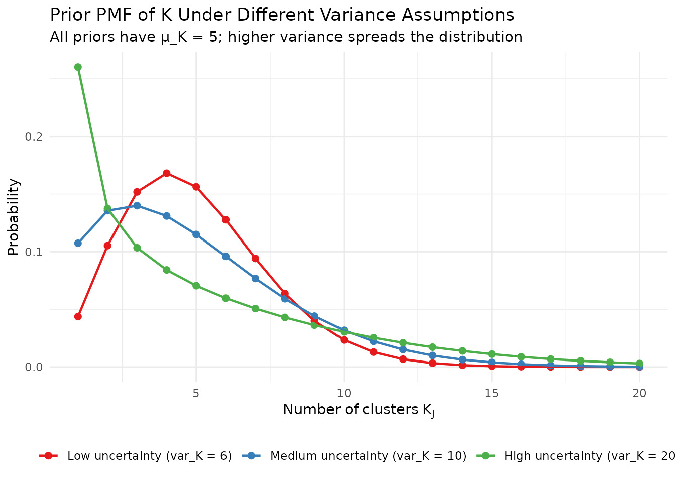
Comparison of K distributions under different variance assumptions.
7. Diagnostic-Driven Refinement
The diagnostic tools enable an iterative workflow for refining your prior until it matches your intentions across all dimensions.
7.1 The Refinement Workflow
The recommended workflow is:
-
Start with K-only calibration: Use
DPprior_fit()with your expectations about cluster counts - Run diagnostics: Check the implied behavior on , , and dominance
- Identify mismatches: Does any aspect of the prior surprise you?
- Refine: Adjust parameters or use dual-anchor if needed
- Repeat: Until all aspects of the prior match your intentions
7.2 Complete Example: From Problem to Solution
Let us walk through a complete example of diagnostic-driven refinement.
Step 1: Initial K-only prior
# Researcher expects ~5 clusters with moderate uncertainty
fit1 <- DPprior_fit(J = 50, mu_K = 5, var_K = 8)
#> Warning: HIGH DOMINANCE RISK: P(w1 > 0.5) = 48.1% exceeds 40%.
#>   This may indicate unintended prior behavior (Lee, 2026).
#>   Consider using DPprior_dual() for weight-constrained elicitation.
#>   See ?DPprior_diagnostics for interpretation.

cat("Step 1: Initial K-only prior\n")
#> Step 1: Initial K-only prior
cat("Gamma(a =", round(fit1$a, 4), ", b =", round(fit1$b, 4), ")\n\n")
#> Gamma(a = 2.0361 , b = 1.6051 )
Step 2: Run diagnostics
diag1 <- DPprior_diagnostics(fit1)

cat("Step 2: Diagnostics reveal...\n")
#> Step 2: Diagnostics reveal...
cat("  K behavior: E[K] =", round(diag1$K$mean, 2),
    ", Var(K) =", round(diag1$K$var, 2), "✓\n")
#>   K behavior: E[K] = 5 , Var(K) = 8 ✓
cat("  Weight behavior: P(w₁ > 0.5) =",
    round(diag1$weights$prob_exceeds["prob_gt_0.5"], 3), "\n")
#>   Weight behavior: P(w₁ > 0.5) = 0.481
cat("  Dominance risk:", toupper(diag1$weights$dominance_risk), "\n")
#>   Dominance risk: HIGH
Step 3: Identify the problem
plot_w1_prior(fit1)#> Step 3: Problem identification
#> The researcher wanted: ~5 clusters with balanced weights
#> The prior implies: ~5 clusters but high chance of one dominant cluster
#> P(w₁ > 0.5) = 48 % is higher than expected for 'balanced' clusters
The K-only prior shows high dominance risk.
Step 4: Apply dual-anchor refinement
cat("Step 4: Dual-anchor refinement\n")
#> Step 4: Dual-anchor refinement
cat("  Adding constraint: P(w₁ > 0.5) ≤ 0.25\n\n")
#>   Adding constraint: P(w₁ > 0.5) ≤ 0.25

fit2 <- DPprior_dual(
  fit = fit1,
  w1_target = list(prob = list(threshold = 0.5, value = 0.25)),
  lambda = 0.7,
  loss_type = "adaptive",
  verbose = FALSE
)

cat("Refined prior: Gamma(a =", round(fit2$a, 4), ", b =", round(fit2$b, 4), ")\n")
#> Refined prior: Gamma(a = 4.3948 , b = 2.5043 )
Step 5: Re-run diagnostics
diag2 <- DPprior_diagnostics(fit2)

cat("Step 5: Post-refinement diagnostics\n")
#> Step 5: Post-refinement diagnostics
cat("  K behavior: E[K] =", round(diag2$K$mean, 2),
    " (shifted from target of 5)\n")
#>   K behavior: E[K] = 6.3  (shifted from target of 5)
cat("  Weight behavior: P(w₁ > 0.5) =",
    round(diag2$weights$prob_exceeds["prob_gt_0.5"], 3), "✓\n")
#>   Weight behavior: P(w₁ > 0.5) = 0.342 ✓
cat("  Dominance risk:", toupper(diag2$weights$dominance_risk), "✓\n")
#>   Dominance risk: MODERATE ✓
Step 6: Visualize the improvement
# Compare w1 distributions
x_grid <- seq(0.001, 0.999, length.out = 500)
w1_df <- data.frame(
  x = rep(x_grid, 2),
  density = c(
    density_w1(x_grid, fit1$a, fit1$b),
    density_w1(x_grid, fit2$a, fit2$b)
  ),
  Prior = rep(c("K-only (before)", "Dual-anchor (after)"), each = length(x_grid))
)
w1_df$Prior <- factor(w1_df$Prior, levels = c("K-only (before)", "Dual-anchor (after)"))

# Cap extreme densities for visualization
w1_df$density[w1_df$density > 10] <- NA

ggplot(w1_df, aes(x = x, y = density, color = Prior)) +
  geom_line(linewidth = 1, na.rm = TRUE) +
  geom_vline(xintercept = 0.5, linetype = "dashed", color = "gray50") +
  scale_color_manual(values = c("#E41A1C", "#377EB8")) +
  annotate("text", x = 0.52, y = 5, label = "P(w₁ > 0.5)", hjust = 0, color = "gray40") +
  labs(
    x = expression(w[1]),
    y = "Density",
    title = "Weight Distribution: Before and After Dual-Anchor Refinement",
    subtitle = sprintf("P(w₁ > 0.5): Before = %.0f%%, After = %.0f%%",
                       100 * diag1$weights$prob_exceeds["prob_gt_0.5"],
                       100 * diag2$weights$prob_exceeds["prob_gt_0.5"])
  ) +
  coord_cartesian(xlim = c(0, 1), ylim = c(0, 6)) +
  theme_minimal() +
  theme(legend.position = "bottom", legend.title = element_blank())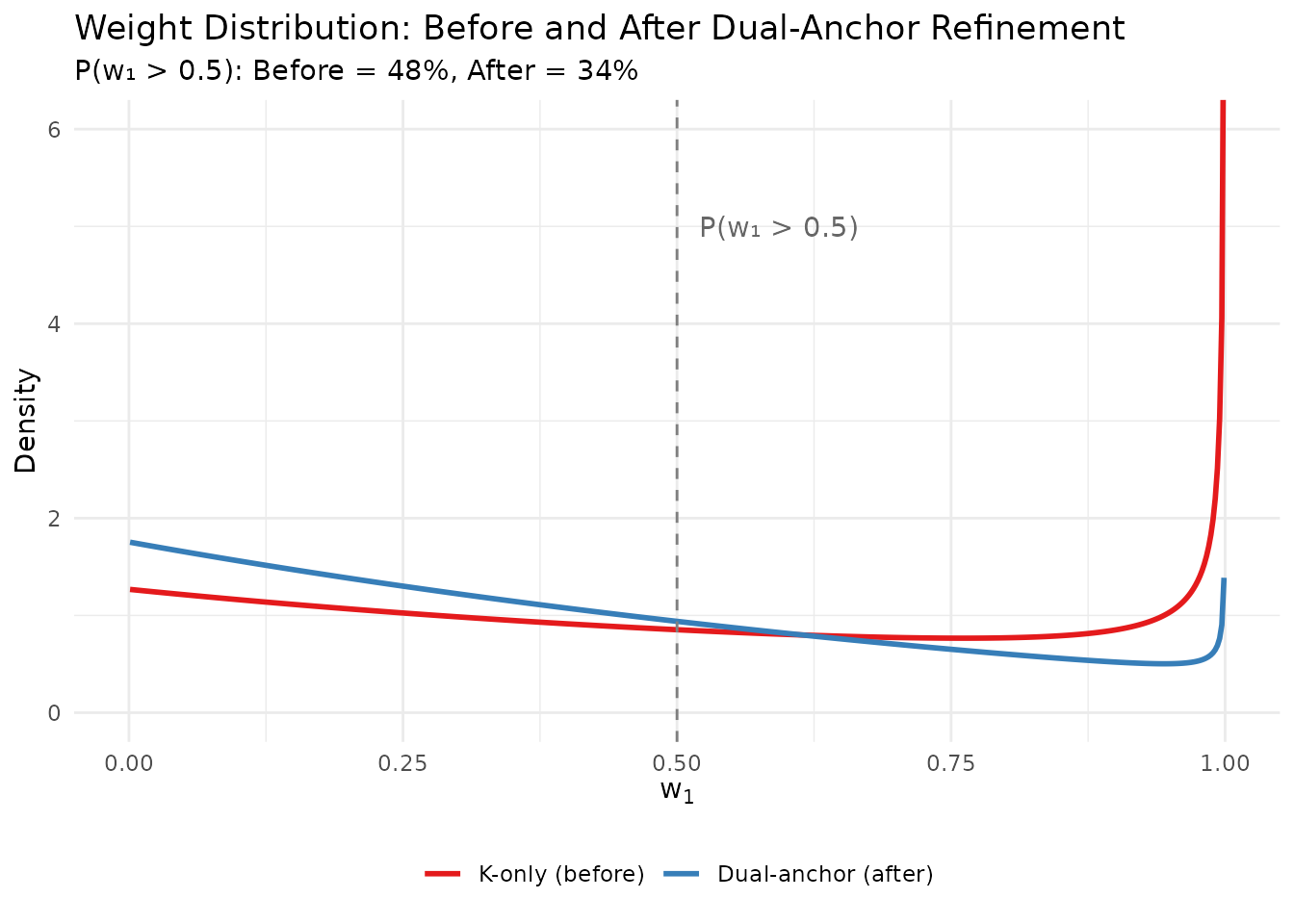
Comparison of weight distributions before and after dual-anchor refinement.
7.3 Summary of the Refinement
comparison_df <- data.frame(
  Metric = c("Gamma(a, b)", "E[K]", "Var(K)", "E[w₁]",
             "P(w₁ > 0.5)", "Dominance Risk"),
  Before = c(
    sprintf("(%.3f, %.3f)", fit1$a, fit1$b),
    sprintf("%.2f", diag1$K$mean),
    sprintf("%.2f", diag1$K$var),
    sprintf("%.3f", diag1$weights$mean),
    sprintf("%.1f%%", 100 * diag1$weights$prob_exceeds["prob_gt_0.5"]),
    toupper(diag1$weights$dominance_risk)
  ),
  After = c(
    sprintf("(%.3f, %.3f)", fit2$a, fit2$b),
    sprintf("%.2f", diag2$K$mean),
    sprintf("%.2f", diag2$K$var),
    sprintf("%.3f", diag2$weights$mean),
    sprintf("%.1f%%", 100 * diag2$weights$prob_exceeds["prob_gt_0.5"]),
    toupper(diag2$weights$dominance_risk)
  )
)

knitr::kable(
  comparison_df,
  col.names = c("Metric", "K-only", "Dual-anchor"),
  caption = "Comparison of prior specifications before and after dual-anchor refinement"
)| Metric | K-only | Dual-anchor |
|---|---|---|
| Gamma(a, b) | (2.036, 1.605) | (4.395, 2.504) |
| E[K] | 5.00 | 6.30 |
| Var(K) | 8.00 | 7.72 |
| E[w₁] | 0.501 | 0.396 |
| P(w₁ > 0.5) | 48.1% | 34.2% |
| Dominance Risk | HIGH | MODERATE |
The trade-off is clear: the refined prior has slightly higher E[K] than the original target of 5, but now has appropriately controlled weight behavior. This is the Pareto trade-off that the dual-anchor framework makes explicit.
8. Comparative Diagnostics
When evaluating multiple candidate priors, comparative diagnostics help you understand the trade-offs.
8.1 Comparing Multiple Priors
# Define three candidate priors
candidates <- list(
  "Conservative" = DPprior_fit(J = 50, mu_K = 5, var_K = 6),
  "Moderate" = DPprior_fit(J = 50, mu_K = 5, var_K = 10),
  "Diffuse" = DPprior_fit(J = 50, mu_K = 5, var_K = 20)
)
#> Warning: HIGH DOMINANCE RISK: P(w1 > 0.5) = 46.5% exceeds 40%.
#>   This may indicate unintended prior behavior (Lee, 2026).
#>   Consider using DPprior_dual() for weight-constrained elicitation.
#>   See ?DPprior_diagnostics for interpretation.
#> Warning: HIGH DOMINANCE RISK: P(w1 > 0.5) = 49.7% exceeds 40%.
#>   This may indicate unintended prior behavior (Lee, 2026).
#>   Consider using DPprior_dual() for weight-constrained elicitation.
#>   See ?DPprior_diagnostics for interpretation.
#> Warning: HIGH DOMINANCE RISK: P(w1 > 0.5) = 56.3% exceeds 40%.
#>   This may indicate unintended prior behavior (Lee, 2026).
#>   Consider using DPprior_dual() for weight-constrained elicitation.
#>   See ?DPprior_diagnostics for interpretation.

# Compute diagnostics for each
comp_results <- lapply(names(candidates), function(nm) {
  fit <- candidates[[nm]]
  diag <- DPprior_diagnostics(fit)
  data.frame(
    Prior = nm,
    a = round(fit$a, 3),
    b = round(fit$b, 3),
    E_K = round(diag$K$mean, 2),
    Var_K = round(diag$K$var, 2),
    E_w1 = round(diag$weights$mean, 3),
    P_w1_gt_50 = sprintf("%.1f%%", 100 * diag$weights$prob_exceeds["prob_gt_0.5"]),
    Risk = toupper(diag$weights$dominance_risk)
  )
})

comp_df <- do.call(rbind, comp_results)

knitr::kable(
  comp_df,
  col.names = c("Prior", "a", "b", "E[K]", "Var(K)", "E[w₁]", "P(w₁>0.5)", "Risk"),
  caption = "Comparative diagnostics for three candidate priors"
)| Prior | a | b | E[K] | Var(K) | E[w₁] | P(w₁>0.5) | Risk |
|---|---|---|---|---|---|---|---|
| Conservative | 3.568 | 2.900 | 5 | 6 | 0.484 | 46.5% | HIGH |
| Moderate | 1.408 | 1.077 | 5 | 10 | 0.518 | 49.7% | HIGH |
| Diffuse | 0.518 | 0.341 | 5 | 20 | 0.585 | 56.3% | HIGH |
8.2 Visualizing the Comparison
# Create comparison data for w1
w1_comp_df <- do.call(rbind, lapply(names(candidates), function(nm) {
  fit <- candidates[[nm]]
  x <- seq(0.001, 0.999, length.out = 300)
  d <- density_w1(x, fit$a, fit$b)
  d[d > 8] <- NA
  data.frame(x = x, density = d, Prior = nm)
}))
w1_comp_df$Prior <- factor(w1_comp_df$Prior, levels = names(candidates))

p1 <- ggplot(w1_comp_df, aes(x = x, y = density, color = Prior)) +
  geom_line(linewidth = 1, na.rm = TRUE) +
  geom_vline(xintercept = 0.5, linetype = "dashed", color = "gray60") +
  scale_color_manual(values = palette_3) +
  coord_cartesian(xlim = c(0, 1), ylim = c(0, 5)) +
  labs(x = expression(w[1]), y = "Density",
       title = expression("Prior on " * w[1])) +
  theme_minimal() +
  theme(legend.position = "bottom", legend.title = element_blank())

# Create comparison data for K
logS <- compute_log_stirling(50)
k_comp_df <- do.call(rbind, lapply(names(candidates), function(nm) {
  fit <- candidates[[nm]]
  pmf <- pmf_K_marginal(50, fit$a, fit$b, logS = logS)
  data.frame(k = seq_along(pmf) - 1, pmf = pmf, Prior = nm)
}))
k_comp_df <- k_comp_df[k_comp_df$k >= 1, ]
k_comp_df$Prior <- factor(k_comp_df$Prior, levels = names(candidates))

p2 <- ggplot(k_comp_df[k_comp_df$k <= 15, ],
             aes(x = k, y = pmf, color = Prior)) +
  geom_point(size = 2) +
  geom_line(linewidth = 0.8) +
  scale_color_manual(values = palette_3) +
  labs(x = expression(K[J]), y = "Probability",
       title = expression("Prior PMF of " * K[J])) +
  theme_minimal() +
  theme(legend.position = "bottom", legend.title = element_blank())

gridExtra::grid.arrange(p1, p2, ncol = 2)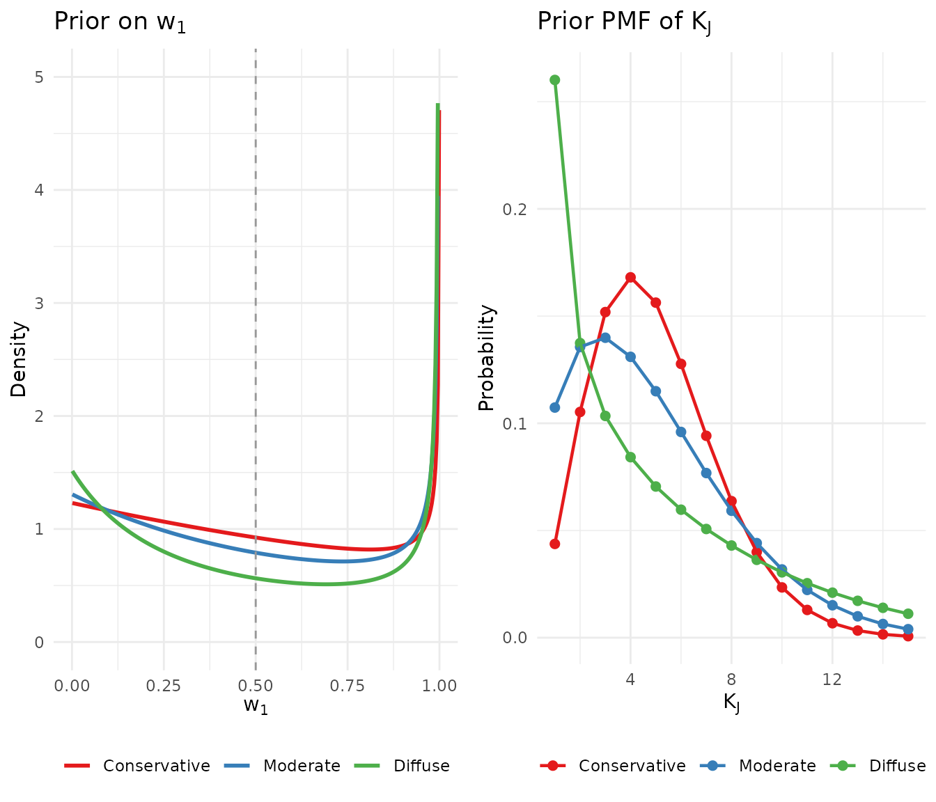
Comparison of three candidate priors across multiple dimensions.
Summary
| Diagnostic Aspect | What to Check | Concern If… |
|---|---|---|
| CV | diag$alpha$cv |
CV > 1 (very diffuse) or CV < 0.3 (very tight) without intention |
| E[K] | diag$K$mean |
Differs substantially from your target |
| Var(K) | diag$K$var |
Differs substantially from your target or implied variance |
| P(w₁ > 0.5) | diag$weights$prob_exceeds["prob_gt_0.5"] |
> 40% without intending high dominance |
| Dominance Risk | diag$weights$dominance_risk |
“high” when you expect balanced clusters |
Key Takeaways:
- Always run diagnostics after eliciting a prior, especially for weight-related quantities
- K-calibration is necessary but not sufficient: matching E[K] does not guarantee intuitive weight behavior
- Use the dominance warning system to catch potential problems early
- Apply dual-anchor refinement when you need to constrain weight behavior explicitly
- Iterate until satisfied: prior elicitation is an iterative process
What’s Next?
Dual-Anchor Framework: Deep dive into controlling both cluster counts and weight behavior
Case Studies: Real-world examples of diagnostic-driven prior refinement
Theory Overview: Mathematical foundations of the diagnostic quantities
References
Lee, J., Che, J., Rabe-Hesketh, S., Feller, A., & Miratrix, L. (2025). Improving the estimation of site-specific effects and their distribution in multisite trials. Journal of Educational and Behavioral Statistics, 50(5), 731–764. https://doi.org/10.3102/10769986241254286
Vicentini, S., & Jermyn, I. H. (2025). Prior selection for the precision parameter of Dirichlet process mixture models. arXiv:2502.00864. https://doi.org/10.48550/arXiv.2502.00864
Sethuraman, J. (1994). A constructive definition of Dirichlet priors. Statistica Sinica, 4(2), 639–650.
For questions or feedback, please visit the GitHub repository.