Case Studies: Multisite Trials and Meta-Analysis

JoonHo Lee (jlee296@ua.edu)

2026-08-22

Overview

This vignette presents three case studies demonstrating how to apply the DPprior package in real-world research contexts. Each case study walks through the complete workflow—from substantive considerations to final prior specification—using published research as a foundation.

The three case studies span different domains and data structures:

Case Study	Domain	J (Sites/Studies)	Key Characteristic
1. Conditional Cash Transfer Trial	Education/Policy	38	Moderate sites, dual-anchor refinement
2. Brief Alcohol Interventions	Public Health	117	Large meta-analysis, multiple heterogeneity sources
3. Alabama Pre-K Value-Added	Education Policy	500 (of 847)	Large-scale policy evaluation

By working through these examples, you will learn how to:

1. Translate substantive domain knowledge into cluster count expectations
2. Choose appropriate calibration methods for different settings
3. Apply diagnostics to verify prior behavior
4. Conduct sensitivity analysis across specifications
5. Report prior elicitation transparently in publications

1. Case Study: Conditional Cash Transfer Multisite Trial

1.1 Research Context

Our first case study draws from the multisite conditional cash transfer (CCT) experiment analyzed in Lee et al. (2025). The Conditional Subsidies for School Attendance program, implemented in Bogotá, Colombia (Barrera-Osorio et al., 2019), conducted randomized experiments across 38 sites in the San Cristobal district.

Study characteristics:

• Sample size: 6,506 participants nested within 38 sites
• Average site size: 171.2 participants
• Coefficient of variation in site sizes: 0.67 (range: 23 to 484)
• Outcomes: Secondary school enrollment and on-time graduation
• Key feature: Large within-site information, limited between-site variation

1.2 The Inferential Goals

The researchers sought to understand the distribution of site-specific treatment effects $\tau_j$, with particular interest in:

1. Estimating the variance of the prior distribution $G$
2. Identifying extreme sites (10th and 90th percentiles)
3. Understanding heterogeneity patterns across sites

Given the estimated cross-site effect standard deviation of $\sigma = 0.04$ to $0.06$ (in effect size units) and relatively high within-site precision, this setting exhibits small between-site information and large within-site information—a configuration where prior choice substantially influences posterior inference.

1.3 Initial Prior Elicitation

Step 1: Determining the expected number of clusters

When eliciting prior beliefs about cluster structure, researchers might consider several substantive factors:

• The intervention was implemented uniformly across sites, suggesting limited structural heterogeneity
• However, local context (school culture, neighborhood characteristics) might create differential responses
• Previous multisite education trials typically exhibit 3–8 distinct response patterns

Based on these considerations, a reasonable expectation is approximately $\mu_K = 5$ clusters among the 38 sites.

# Define the study context
J_cct <- 38
mu_K_cct <- 5

cat("Study context:\n")
#> Study context:
cat("  Number of sites (J):", J_cct, "\n")
#>   Number of sites (J): 38
cat("  Expected clusters (μ_K):", mu_K_cct, "\n")
#>   Expected clusters (μ_K): 5
cat("  Ratio (μ_K/J):", round(mu_K_cct / J_cct, 3), "\n")
#>   Ratio (μ_K/J): 0.132

Step 2: Expressing uncertainty

Given the novelty of this specific intervention context and the moderate sample of sites, we should express substantial uncertainty. A “low” confidence level is appropriate:

# Initial fit with a reviewable low-confidence target
target_cct <- DPprior_target_K(
  J = J_cct, mu_K = mu_K_cct, confidence = "low"
)
fit_cct <- DPprior_fit(
  J = J_cct,
  target_K = target_cct,
  method = "A2-MN",
  M = 160L,
  check_diagnostics = FALSE
)

print(fit_cct)
#> DPprior Prior Elicitation Result
#> ============================================= 
#> 
#> Schema: dpprior.result/1
#> Method: A2-MN (mode: a2_moment)
#> Status: converged; usable: yes; verified: yes
#> 
#> Target (J = 38):
#>   E[K_J]   = 5.0000
#>   Var(K_J) = 20.0000
#> 
#> Canonical candidate:
#>   alpha ~ Gamma(a = 0.4629, b = 0.2556)
#>   Achieved E[K_J] = 5.000000; Var(K_J) = 20.000000
#>   Maximum absolute moment residual = 3.05e-10
#> 
#> Canonical guidance: scaled component residuals and independent higher-order verification passed

1.4 Comprehensive Diagnostics

Before accepting this prior, we need to verify its behavior across multiple dimensions. The DPprior_diagnostics() function provides a comprehensive assessment:

# This low-confidence case can require an explicitly reviewable approximate
# diagnostic bundle; its status quartet is reported below rather than upgraded.
diag_cct <- DPprior_diagnostics(fit_cct, allow_approximate = TRUE)
alpha_cct <- diag_cct$diagnostics$alpha
K_cct <- diag_cct$diagnostics$K
wsb_cct <- diag_cct$diagnostics$weights
rho_cct <- diag_cct$diagnostics$coclustering
alpha_sd_cct <- sqrt(fit_cct$parameters$a) / fit_cct$parameters$b
alpha_q_cct <- qgamma(
  c(q5 = 0.05, q50 = 0.50, q95 = 0.95),
  shape = fit_cct$parameters$a, rate = fit_cct$parameters$b
)
K_mode_cct <- which.max(K_cct$pmf)
wsb_median_cct <- quantile_w1(
  0.5, fit_cct$parameters$a, fit_cct$parameters$b
)
wsb_tail_cct <- c(
  threshold_0.5 = prob_wsb_exceeds(
    0.5, fit_cct$parameters$a, fit_cct$parameters$b
  ),
  threshold_0.9 = prob_wsb_exceeds(
    0.9, fit_cct$parameters$a, fit_cct$parameters$b
  )
)

cat("=== Comprehensive Diagnostic Report ===\n\n")
#> === Comprehensive Diagnostic Report ===

cat("1. ALPHA DISTRIBUTION\n")
#> 1. ALPHA DISTRIBUTION
cat("   Mean:     ", round(alpha_cct$mean, 3), "\n")
#>    Mean:      1.811
cat("   SD:       ", round(alpha_sd_cct, 3), "\n")
#>    SD:        2.662
cat("   CV:       ", round(alpha_cct$CV, 3), "\n")
#>    CV:        1.47
cat("   5th %ile: ", round(alpha_q_cct["q5"], 3), "\n")
#>    5th %ile:  0.005
cat("   50th %ile:", round(alpha_q_cct["q50"], 3), "\n")
#>    50th %ile: 0.767
cat("   95th %ile:", round(alpha_q_cct["q95"], 3), "\n")
#>    95th %ile: 7.15

cat("\n2. CLUSTER COUNT (K)\n")
#> 
#> 2. CLUSTER COUNT (K)
cat("   E[K]:     ", round(K_cct$mean, 3), "\n")
#>    E[K]:      5
cat("   Var(K):   ", round(K_cct$variance, 3), "\n")
#>    Var(K):    20
cat("   SD(K):    ", round(sqrt(K_cct$variance), 3), "\n")
#>    SD(K):     4.472
cat("   Mode(K):  ", K_mode_cct, "\n")
#>    Mode(K):   1

cat("\n3. WEIGHT BEHAVIOR\n")
#> 
#> 3. WEIGHT BEHAVIOR
cat("   E[W_SB]:        ", round(wsb_cct$mean, 3), "\n")
#>    E[W_SB]:         0.572
cat("   Median(W_SB):   ", round(wsb_median_cct, 3), "\n")
#>    Median(W_SB):    0.588
cat("   P(W_SB > 0.5):  ",
    round(wsb_tail_cct["threshold_0.5"], 3), "\n")
#>    P(W_SB > 0.5):   0.545
cat("   P(W_SB > 0.9):  ",
    round(wsb_tail_cct["threshold_0.9"], 3), "\n")
#>    P(W_SB > 0.9):   0.344
cat("   W_SB status:    ", wsb_cct$status, "\n")
#>    W_SB status:     converged

cat("\n4. CO-CLUSTERING PROBABILITY (ρ)\n")
#> 
#> 4. CO-CLUSTERING PROBABILITY (ρ)
cat("   E[ρ]:         ", round(rho_cct$mean, 3), "\n")
#>    E[ρ]:          0.572
cat("   Interpretation: Two random sites have a", 
    round(100 * rho_cct$mean), "% chance of sharing a cluster\n")
#>    Interpretation: Two random sites have a 57 % chance of sharing a cluster
cat("\nBundle status:\n")
#> 
#> Bundle status:
print(diag_cct[c("status", "usable", "verified", "message")])
#> $status
#> [1] "approximate"
#> 
#> $usable
#> [1] FALSE
#> 
#> $verified
#> [1] FALSE
#> 
#> $message
#> [1] "At least one canonical diagnostic component did not pass the fixed refinement contract."

1.5 Visualizing the Initial Prior

The DPprior package provides several visualization functions to help understand prior behavior. Let’s examine each component:

Alpha distribution:

plot_alpha_prior(fit_cct)

Prior distribution on the concentration parameter α for the CCT study.

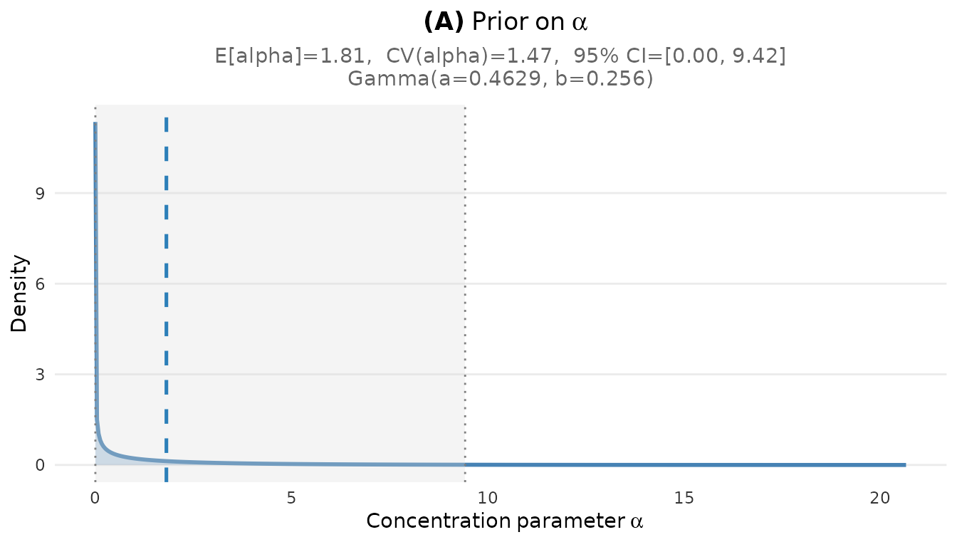
Prior distribution on the concentration parameter α for the CCT study.

Cluster count distribution:

plot_K_prior(fit_cct)

Prior PMF of the number of clusters K for the CCT study (J = 38).

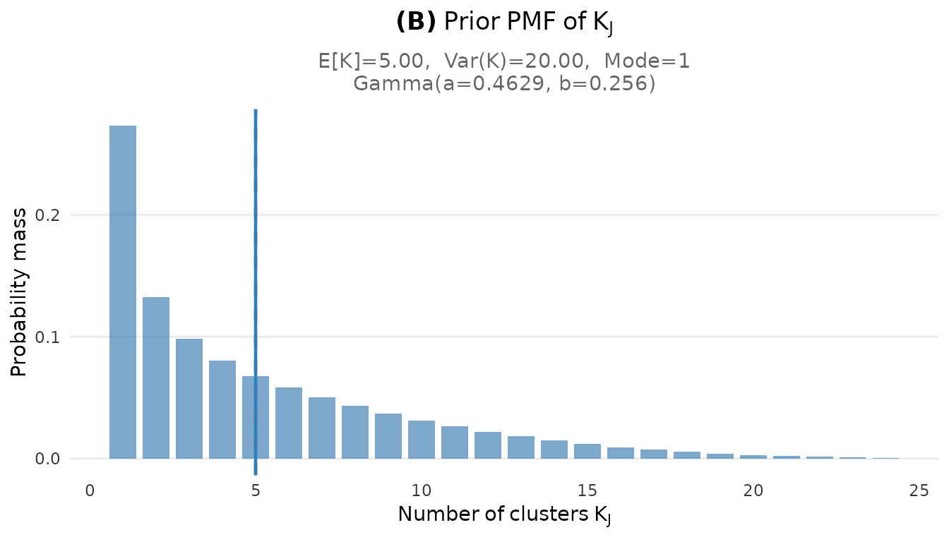
Prior PMF of the number of clusters K for the CCT study (J = 38).

First size-biased weight distribution:

plot_w1_prior(fit_cct)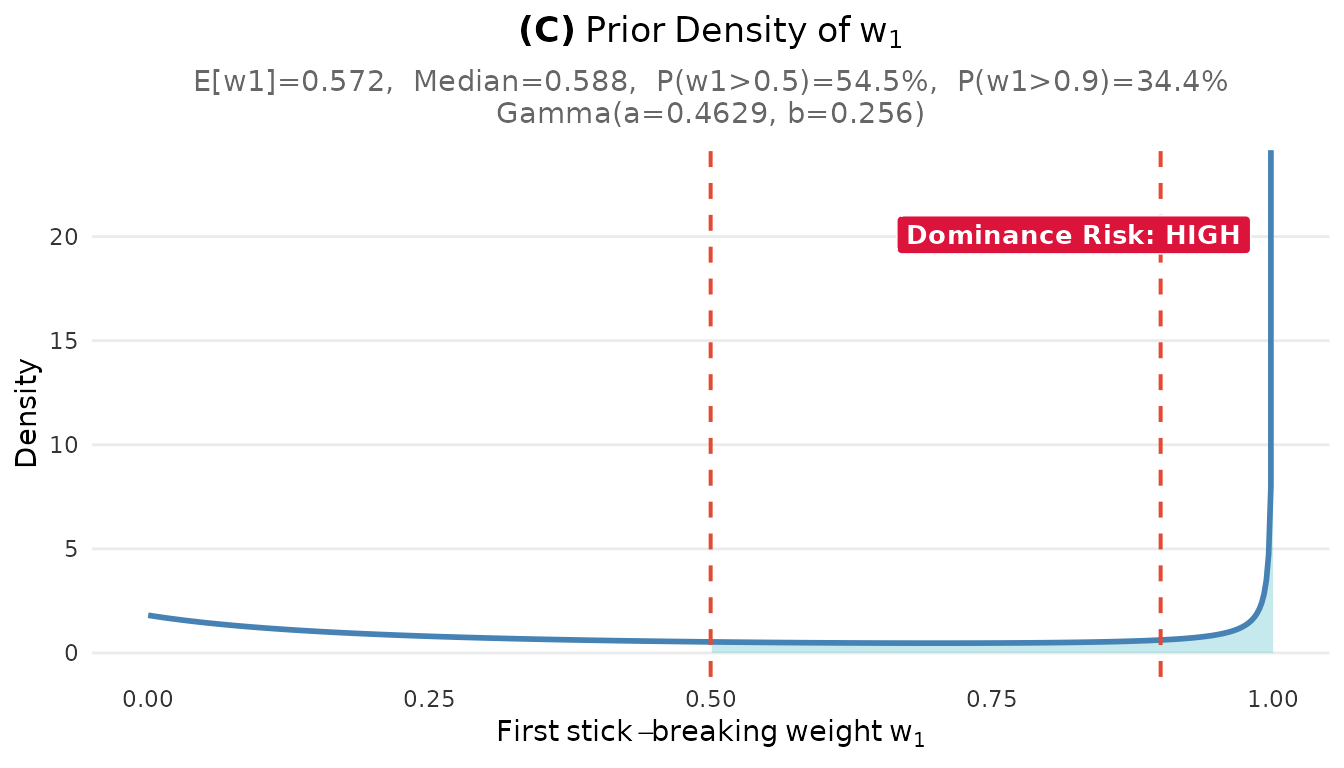

Prior distribution of the first size-biased weight W_SB. The dashed line marks the reviewed mass threshold 0.5.

Prior distribution of the first size-biased weight W_SB. The dashed line marks the reviewed mass threshold 0.5.

Complete dashboard:

plot(fit_cct)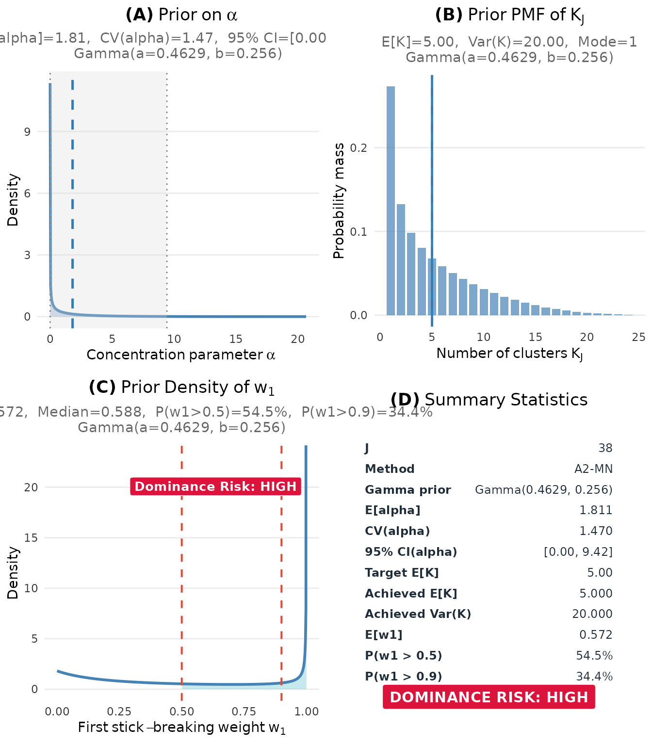

Complete prior elicitation dashboard for the CCT multisite trial (J = 38, μ_K = 5).

#> TableGrob (2 x 2) "dpprior_dashboard": 4 grobs
#>   z     cells              name           grob
#> 1 1 (1-1,1-1) dpprior_dashboard gtable[layout]
#> 2 2 (2-2,1-1) dpprior_dashboard gtable[layout]
#> 3 3 (1-1,2-2) dpprior_dashboard gtable[layout]
#> 4 4 (2-2,2-2) dpprior_dashboard gtable[layout]

1.6 Addressing a Large $W_{SB}$ Tail Probability

The diagnostics reveal an important concern: the named tail probability $P(W_{SB}>0.5)=0.54$. This means there is a 54% prior probability that the size-biased first stick-breaking cluster mass exceeds one half.

In a setting with limited between-site information, this large $P(W_{SB}>0.5)$ can lead to overshrinkage in posterior inference. The dual-anchor framework allows us to constrain that named tail probability while maintaining our beliefs about the expected number of clusters.

Applying dual-anchor refinement:

We require $P(W_{SB} > 0.5) \leq 0.25$ while keeping $K$ as the optimization objective while independently certifying the weight inequality:

# Apply a verified hard bound to the named W_SB tail probability
fit_cct_dual <- DPprior_dual_hard(
  fit = fit_cct,
  constraint = list(
    metric = "wsb_tail", threshold = 0.5,
    relation = "<=", bound = 0.25
  )
)

cat("Original prior:    Gamma(a =", round(fit_cct$parameters$a, 4),
    ", b =", round(fit_cct$parameters$b, 4), ")\n")
#> Original prior:    Gamma(a = 0.4629 , b = 0.2556 )
cat("Dual-anchor prior: Gamma(a =", round(fit_cct_dual$parameters$a, 4),
    ", b =", round(fit_cct_dual$parameters$b, 4), ")\n")
#> Dual-anchor prior: Gamma(a = 1.8148 , b = 0.6045 )
cat("Constraint verified:", fit_cct_dual$constraint$satisfied, "\n")
#> Constraint verified: TRUE
fit_cct_dual[c("status", "usable", "verified", "message")]
#> $status
#> [1] "boundary"
#> 
#> $usable
#> [1] TRUE
#> 
#> $verified
#> [1] TRUE
#> 
#> $message
#> [1] "Hard inequality solution passed verification with the constraint active."

Verifying the improvement:

# The hard-fit object already carries its verified K and named weight evidence.
K_cct_dual <- fit_cct_dual$achieved$K
alpha_mean_cct_dual <- with(
  fit_cct_dual$parameters, a / b
)
wsb_mean_cct_dual <- mean_w1(
  fit_cct_dual$parameters$a, fit_cct_dual$parameters$b
)
wsb_tail_cct_dual <- fit_cct_dual$achieved$weight$value

# Create comparison table
comparison_df <- data.frame(
  Metric = c(
    "E[α]", "E[K]", "Var(K)", "E[W_SB]", "P(W_SB > 0.5)",
    "Diagnostic status"
  ),
  Original = c(
    round(alpha_cct$mean, 3),
    round(K_cct$mean, 2),
    round(K_cct$variance, 2),
    round(wsb_cct$mean, 3),
    round(wsb_tail_cct["threshold_0.5"], 3),
    diag_cct$status
  ),
  Dual_Anchor = c(
    round(alpha_mean_cct_dual, 3),
    round(K_cct_dual$mean, 2),
    round(K_cct_dual$variance, 2),
    round(wsb_mean_cct_dual, 3),
    round(wsb_tail_cct_dual, 3),
    fit_cct_dual$status
  )
)

knitr::kable(
  comparison_df,
  col.names = c("Metric", "K-only Prior", "Dual-Anchor Prior"),
  caption = "Comparison of K-only and dual-anchor priors for the CCT study"
)

Comparison of K-only and dual-anchor priors for the CCT study

Metric	K-only Prior	Dual-Anchor Prior
E[α]	1.811	3.002
E[K]	5	7.72
Var(K)	20	15.98
E[W_SB]	0.572	0.329
P(W_SB > 0.5)	0.545	0.25
Diagnostic status	approximate	boundary

1.7 Comparing K-only vs Dual-Anchor Priors

Let’s visualize the difference between the two priors:

# Prepare data for K PMF comparison
logS_cct <- compute_log_stirling(J_cct)

pmf_original <- pmf_K_marginal(
  J_cct, fit_cct$parameters$a, fit_cct$parameters$b, logS = logS_cct
)
pmf_dual <- pmf_K_marginal(
  J_cct, fit_cct_dual$parameters$a, fit_cct_dual$parameters$b,
  logS = logS_cct
)

k_compare_df <- data.frame(
  K = rep(seq_along(pmf_original), 2),
  Probability = c(pmf_original, pmf_dual),
  Prior = rep(c("K-only", "Dual-anchor"), each = length(pmf_original))
)
k_compare_df$Prior <- factor(k_compare_df$Prior, levels = c("K-only", "Dual-anchor"))

# Prepare data for w1 comparison
w1_grid <- seq(0, 1, length.out = 200)
w1_dens_original <- sapply(w1_grid, function(w) {
  density_w1(w, fit_cct$parameters$a, fit_cct$parameters$b)
})
w1_dens_dual <- sapply(w1_grid, function(w) {
  density_w1(w, fit_cct_dual$parameters$a, fit_cct_dual$parameters$b)
})

w1_compare_df <- data.frame(
  w1 = rep(w1_grid, 2),
  Density = c(w1_dens_original, w1_dens_dual),
  Prior = rep(c("K-only", "Dual-anchor"), each = length(w1_grid))
)
w1_compare_df$Prior <- factor(w1_compare_df$Prior, levels = c("K-only", "Dual-anchor"))

# Create plots
p1 <- ggplot(k_compare_df[k_compare_df$K <= 15, ], 
             aes(x = K, y = Probability, fill = Prior)) +
  geom_col(position = "dodge", alpha = 0.8) +
  scale_fill_manual(values = palette_2) +
  labs(
    x = expression(K[J]),
    y = "Probability",
    title = "Cluster Count Distribution"
  ) +
  theme_minimal() +
  theme(legend.position = "bottom", legend.title = element_blank())

p2 <- ggplot(w1_compare_df, aes(x = w1, y = Density, color = Prior)) +
  geom_line(linewidth = 1) +
  geom_vline(xintercept = 0.5, linetype = "dashed", color = "gray50") +
  scale_color_manual(values = palette_2) +
  labs(
    x = expression(w[1]),
    y = "Density",
    title = "First Size-Biased Weight Distribution"
  ) +
  theme_minimal() +
  theme(legend.position = "bottom", legend.title = element_blank())

gridExtra::grid.arrange(p1, p2, ncol = 2)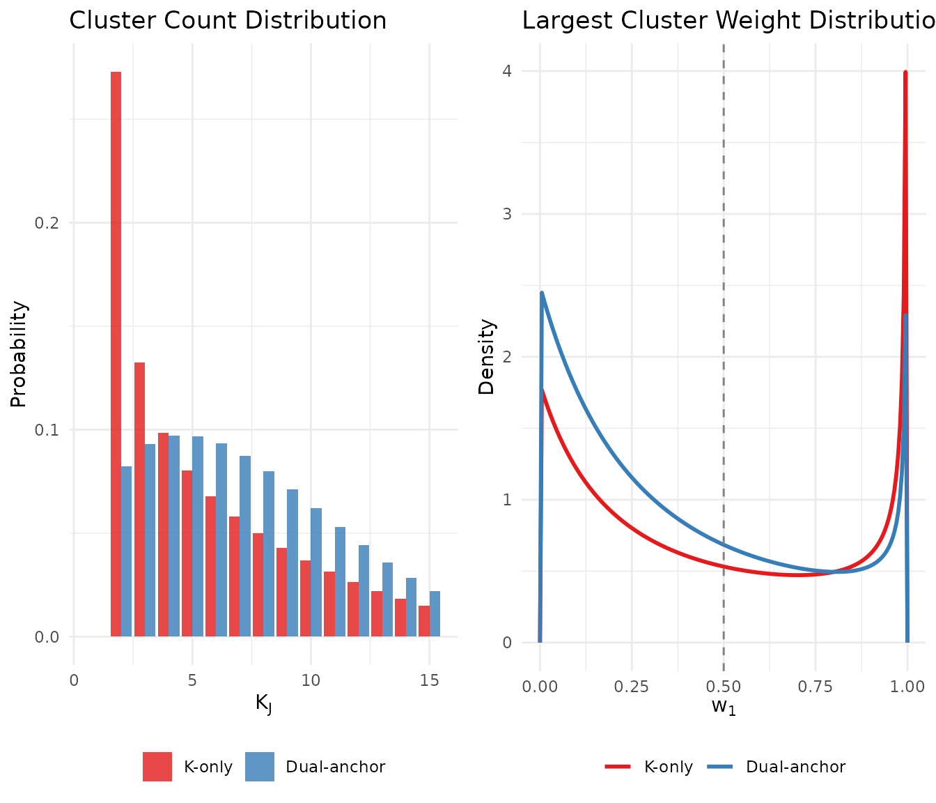

Comparison of K-only and dual-anchor priors: the dual-anchor approach reduces P(W_SB > 0.5) while maintaining similar cluster count expectations.

The dual-anchor prior shifts mass in the $W_{SB}$ distribution away from extreme values (right panel) while maintaining a similar expected number of clusters (left panel). This reduces the named tail probability without substantially changing our beliefs about cluster count.

1.8 Sensitivity Analysis

Given the uncertainty in our prior specification, we conduct a sensitivity analysis across a range of plausible values for both the K-only and dual-anchor approaches:

# Sensitivity to μ_K
mu_K_grid <- c(3, 5, 7, 9)

sensitivity_results <- lapply(mu_K_grid, function(mu) {
  # K-only fit
  target_k <- DPprior_target_K(J = J_cct, mu_K = mu, confidence = "low")
  fit_k <- DPprior_fit(
    J = J_cct, target_K = target_k, method = "A2-MN", M = 160L,
    check_diagnostics = FALSE
  )
  diag_k <- DPprior_diagnostics(fit_k, allow_approximate = TRUE)
  
  # Verified hard dual-anchor fit
  fit_d <- DPprior_dual_hard(
    fit = fit_k,
    constraint = list(
      metric = "wsb_tail", threshold = 0.5,
      relation = "<=", bound = 0.25
    )
  )
  K_k <- diag_k$diagnostics$K
  K_d <- fit_d$achieved$K
  
  data.frame(
    mu_K = mu,
    # K-only results
    a_k = round(fit_k$parameters$a, 3),
    b_k = round(fit_k$parameters$b, 3),
    E_K_k = round(K_k$mean, 2),
    P_WSB_k = round(prob_wsb_exceeds(
      0.5, fit_k$parameters$a, fit_k$parameters$b
    ), 3),
    # Dual-anchor results
    a_d = round(fit_d$parameters$a, 3),
    b_d = round(fit_d$parameters$b, 3),
    E_K_d = round(K_d$mean, 2),
    P_WSB_d = round(fit_d$achieved$weight$value, 3)
  )
})

sensitivity_df <- do.call(rbind, sensitivity_results)

knitr::kable(
  sensitivity_df,
  col.names = c("Target μ_K", 
                "a (K)", "b (K)", "E[K]", "P(W_SB>0.5)",
                "a (DA)", "b (DA)", "E[K]", "P(W_SB>0.5)"),
  row.names = FALSE,
  caption = "Sensitivity analysis: K-only (K) vs Dual-anchor (DA) priors (J = 38, low confidence)"
)

Sensitivity analysis: K-only (K) vs Dual-anchor (DA) priors (J = 38, low confidence)

Target μ_K	a (K)	b (K)	E[K]	P(W_SB>0.5)	a (DA)	b (DA)	E[K]	P(W_SB>0.5)
3	0.270	0.345	3	0.743	11.839	5.580	6.67	0.25
5	0.463	0.256	5	0.545	1.815	0.605	7.72	0.25
7	0.601	0.191	7	0.399	1.084	0.268	8.71	0.25
9	0.694	0.143	9	0.293	0.816	0.155	9.62	0.25

1.9 Final Prior Selection and Reporting

Based on our analysis, we recommend the dual-anchor prior for the CCT study, as it provides appropriate control over the predeclared $W_{SB}$ tail probability in this low between-site information setting.

cat("RECOMMENDED PRIOR FOR CCT STUDY\n")
#> RECOMMENDED PRIOR FOR CCT STUDY
cat("================================\n")
#> ================================
cat("α ~ Gamma(", round(fit_cct_dual$parameters$a, 4), ", ",
    round(fit_cct_dual$parameters$b, 4), ")\n\n", sep = "")
#> α ~ Gamma(1.8148, 0.6045)
cat("Key properties:\n")
#> Key properties:
cat("  E[K] =", round(K_cct_dual$mean, 2), "clusters\n")
#>   E[K] = 7.72 clusters
cat("  P(W_SB > 0.5) =",
    round(wsb_tail_cct_dual, 2), "\n")
#>   P(W_SB > 0.5) = 0.25
cat("  Hard constraint verified:", fit_cct_dual$constraint$satisfied, "\n")
#>   Hard constraint verified: TRUE

Reporting language for publication:

We elicited beliefs about the number of latent clusters among the $J = 38$ sites in the CCT multisite trial. Based on substantive knowledge of similar education interventions and the uniformity of implementation, we specified $\mathbb{E}[K_J] = 5$ (approximately five distinct response patterns) with low confidence. Initial diagnostics using the K-only calibration yielded $P(W_{SB} > 0.5) = 0.54$, which is problematic in settings with limited between-site information. We therefore applied verified hard dual-anchor refinement with $P(W_{SB} > 0.5) \leq 0.25$, yielding a Gamma(1.815, 0.605) hyperprior. The refined prior maintains $\mathbb{E}[K_J] \approx 7.7$ while independently verifying the declared weight inequality. Sensitivity analyses across $\mu_K \in \{3, 5, 7, 10\}$ confirmed that substantive conclusions were robust to prior specification.

2. Case Study: Brief Alcohol Interventions Meta-Analysis

2.1 Research Context

Our second case study is based on the meta-analysis of brief alcohol interventions (BAI) for adolescents and young adults conducted by Pustejovsky & Tipton (2022), who re-analyzed data from Tanner-Smith & Lipsey (2015).

Study characteristics:

• Number of studies: 117 randomized trials
• Total effect sizes: 1,198 estimates
• Effect sizes per study: Median = 6, range = 1 to 108
• Outcome: Alcohol consumption (standardized mean differences)
• Key feature: Complex dependence structure (correlated and hierarchical)

2.2 The Meta-Analytic Challenge

In meta-analysis, the Dirichlet Process mixture model can be used to flexibly model the distribution of true study effects. This is particularly valuable when:

• The true effect distribution may be non-Gaussian
• There may be discrete subpopulations of studies with similar effects
• Robust inference is needed without strong distributional assumptions

The BAI meta-analysis presents a setting with substantial between-study heterogeneity ($\hat{\tau} = 0.182$ under the correlated effects model), suggesting the potential for distinct effect subgroups.

2.3 Eliciting the Prior

Step 1: Substantive reasoning about clusters

In the BAI context, we consider potential sources of effect heterogeneity:

• Intervention type: Brief motivational interviewing vs. feedback-only vs. multi-session programs vs. computerized interventions
• Population: College students vs. high school vs. clinical samples vs. community populations
• Outcome timing: Immediate vs. short-term (3 months) vs. medium-term (6 months) vs. long-term (12+ months) effects
• Control condition: No treatment vs. attention control vs.  treatment-as-usual vs. alternative intervention
• Delivery format: Individual vs. group vs. self-administered
• Setting: Healthcare vs. educational vs. community

Given the many potential mechanisms for heterogeneity and the large number of studies, a reasonable expectation might be 15–25 distinct effect clusters among 117 studies. We start with $\mu_K = 18$:

# Define the meta-analysis context
J_bai <- 117
mu_K_bai <- 18

cat("Meta-analysis context:\n")
#> Meta-analysis context:
cat("  Number of studies (J):", J_bai, "\n")
#>   Number of studies (J): 117
cat("  Expected clusters (μ_K):", mu_K_bai, "\n")
#>   Expected clusters (μ_K): 18
cat("  Ratio (μ_K/J):", round(mu_K_bai / J_bai, 3), "\n")
#>   Ratio (μ_K/J): 0.154

Step 2: Expressing uncertainty

Meta-analyses often have more uncertainty about the number of distinct effect clusters than multisite trials, as studies are conducted independently with varying methodologies. We use low confidence:

target_bai <- DPprior_target_K(
  J = J_bai, mu_K = mu_K_bai, confidence = "low"
)
fit_bai <- DPprior_fit(
  J = J_bai,
  target_K = target_bai,
  method = "A2-MN",
  M = 160L,
  check_diagnostics = FALSE
)

print(fit_bai)
#> DPprior Prior Elicitation Result
#> ============================================= 
#> 
#> Schema: dpprior.result/1
#> Method: A2-MN (mode: a2_moment)
#> Status: converged; usable: yes; verified: yes
#> 
#> Target (J = 117):
#>   E[K_J]   = 18.0000
#>   Var(K_J) = 85.0000
#> 
#> Canonical candidate:
#>   alpha ~ Gamma(a = 1.9005, b = 0.2986)
#>   Achieved E[K_J] = 18.000000; Var(K_J) = 85.000000
#>   Maximum absolute moment residual = 5.17e-08
#> 
#> Canonical guidance: scaled component residuals and independent higher-order verification passed

Step 3: Diagnostic verification

diag_bai <- DPprior_diagnostics(fit_bai, allow_approximate = TRUE)
alpha_bai <- diag_bai$diagnostics$alpha
K_bai <- diag_bai$diagnostics$K
wsb_bai <- diag_bai$diagnostics$weights
alpha_sd_bai <- sqrt(fit_bai$parameters$a) / fit_bai$parameters$b
alpha_q_bai <- qgamma(
  c(q5 = 0.05, q95 = 0.95),
  shape = fit_bai$parameters$a, rate = fit_bai$parameters$b
)
K_mode_bai <- which.max(K_bai$pmf)
wsb_tail_bai <- prob_wsb_exceeds(
  0.5, fit_bai$parameters$a, fit_bai$parameters$b
)

cat("Diagnostic Summary:\n")
#> Diagnostic Summary:
cat("----------------\n")
#> ----------------
cat("Alpha distribution:\n")
#> Alpha distribution:
cat("  E[α] =", round(alpha_bai$mean, 3), "\n")
#>   E[α] = 6.365
cat("  SD(α) =", round(alpha_sd_bai, 3), "\n")
#>   SD(α) = 4.617
cat("  90% central interval: [", round(alpha_q_bai["q5"], 3), ", ",
    round(alpha_q_bai["q95"], 3), "]\n", sep = "")
#>   90% central interval: [1.059, 15.344]
cat("\nCluster count:\n")
#> 
#> Cluster count:
cat("  E[K] =", round(K_bai$mean, 3), "\n")
#>   E[K] = 18
cat("  Var(K) =", round(K_bai$variance, 3), "\n")
#>   Var(K) = 85
cat("  Mode(K) =", K_mode_bai, "\n")
#>   Mode(K) = 14
cat("\nWeight behavior:\n")
#> 
#> Weight behavior:
cat("  E[W_SB] =", round(wsb_bai$mean, 3), "\n")
#>   E[W_SB] = 0.2
cat("  P(W_SB > 0.5) =",
    round(wsb_tail_bai, 3), "\n")
#>   P(W_SB > 0.5) = 0.102
print(diag_bai[c("status", "usable", "verified", "message")])
#> $status
#> [1] "converged"
#> 
#> $usable
#> [1] TRUE
#> 
#> $verified
#> [1] TRUE
#> 
#> $message
#> [1] "All canonical diagnostic components passed independent selected-versus-verifier checks."

2.4 Comparing Alternative Specifications

For meta-analysis, it is valuable to compare different prior specifications to assess robustness. We compare three approaches: expecting fewer clusters, the baseline, and expecting more clusters.

# Define three candidate priors
fit_bai_candidate <- function(mu_K) {
  target_K <- DPprior_target_K(
    J = J_bai, mu_K = mu_K, confidence = "low"
  )
  DPprior_fit(
    J = J_bai, target_K = target_K, method = "A2-MN", M = 160L,
    check_diagnostics = FALSE
  )
}
bai_candidates <- list(
  "Conservative (μ_K = 10)" = fit_bai_candidate(10),
  "Baseline (μ_K = 18)" = fit_bai_candidate(18),
  "Liberal (μ_K = 30)" = fit_bai_candidate(30)
)

# Create comparison table
bai_comp_results <- lapply(names(bai_candidates), function(nm) {
  fit <- bai_candidates[[nm]]
  diag <- DPprior_diagnostics(fit, allow_approximate = TRUE)
  K_diag <- diag$diagnostics$K
  wsb_diag <- diag$diagnostics$weights
  rho_diag <- diag$diagnostics$coclustering
  data.frame(
    Prior = nm,
    a = round(fit$parameters$a, 3),
    b = round(fit$parameters$b, 3),
    E_K = round(K_diag$mean, 2),
    E_w1 = round(wsb_diag$mean, 3),
    E_rho = round(rho_diag$mean, 3),
    Status = diag$status,
    Verified = diag$verified
  )
})

bai_comp_df <- do.call(rbind, bai_comp_results)

knitr::kable(
  bai_comp_df,
  col.names = c(
    "Prior", "a", "b", "E[K]", "E[W_SB]", "E[ρ]",
    "Status", "Verified"
  ),
  caption = "Comparison of candidate priors for the BAI meta-analysis (J = 117)"
)

Comparison of candidate priors for the BAI meta-analysis (J = 117)

Prior	a	b	E[K]	E[W_SB]	E[ρ]	Status	Verified
Conservative (μ_K = 10)	1.232	0.449	10	0.379	0.379	converged	TRUE
Baseline (μ_K = 18)	1.901	0.299	18	0.200	0.200	converged	TRUE
Liberal (μ_K = 30)	2.470	0.173	30	0.096	0.096	approximate	FALSE

2.5 Visualizing the Comparison

# Create data for K PMF comparison
logS_bai <- compute_log_stirling(J_bai)

k_bai_df <- do.call(rbind, lapply(names(bai_candidates), function(nm) {
  fit <- bai_candidates[[nm]]
  pmf <- pmf_K_marginal(
    J_bai, fit$parameters$a, fit$parameters$b, logS = logS_bai
  )
  data.frame(
    K = seq_along(pmf),
    probability = pmf,
    Prior = nm
  )
}))
k_bai_df$Prior <- factor(k_bai_df$Prior, levels = names(bai_candidates))

# Plot PMF comparison
ggplot(k_bai_df[k_bai_df$K <= 50, ], 
       aes(x = K, y = probability, color = Prior)) +
  geom_line(linewidth = 0.8) +
  geom_point(size = 1.5) +
  scale_color_manual(values = palette_3) +
  labs(
    x = expression(K[J]),
    y = "Probability",
    title = "Prior PMF of Number of Clusters (BAI Meta-Analysis)",
    subtitle = "J = 117 studies"
  ) +
  theme_minimal() +
  theme(legend.position = "bottom", legend.title = element_blank())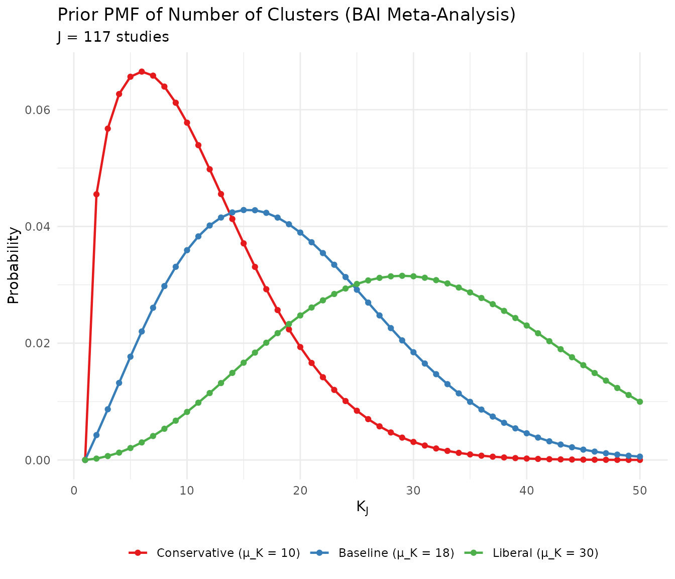

Comparison of three candidate priors for the BAI meta-analysis.

3. Case Study: Alabama Pre-K Value-Added Analysis

3.1 Research Context

Our third case study illustrates prior elicitation for a large-scale value-added analysis in Alabama’s pre-kindergarten program.

Study characteristics:

• Sites: 847 pre-K sites across the state
• Providers: 74.4% public schools, 10.4% private centers, 6.2% Head Start, and others
• Class sizes: 13–18 students per classroom
• Outcomes: Six developmental domains (Literacy, Mathematics, Cognitive, Language, Social-Emotional, Physical)
• Assessment: Teaching Strategies GOLD®

A note on package limitations: The current version of DPprior supports $J \leq 500$ due to pre-computed unsigned Stirling numbers of the first kind, which are required for exact moment calculations. Support for larger $J$ is planned for future releases. For the 847 sites in the Alabama study, we demonstrate the workflow using $J = 500$ as a practical upper bound. This limitation has minimal impact on substantive conclusions for several reasons: (1) the relationship between $\alpha$ and $\mathbb{E}[K_J]$ is approximately logarithmic in $J$, so results are relatively stable across nearby sample sizes; (2) using a conservative (smaller) $J$ tends to produce slightly more concentrated priors, which is a defensible choice in uncertain settings; and (3) the $\mu_K / J$ ratio—rather than $J$ alone—is the primary driver of the elicited prior.

3.2 The Value-Added Challenge

Value-added models (VAMs) estimate site-specific contributions to student learning ($\theta_j$). Key challenges in this context include:

1. Distribution estimation: Is the distribution of site effects normal, or are there distinct subpopulations?
2. Tail identification: Which sites fall in the lowest and highest 10% of the distribution?
3. Ranking: Can we produce meaningful “report cards” for sites?

The semiparametric Dirichlet Process approach allows flexible modeling of the site effect distribution without imposing normality.

3.3 Eliciting the Prior

Step 1: Substantive considerations

With 847 sites, we expect considerable heterogeneity. Potential sources of clustering include:

• Provider type: Public schools vs. private centers vs. Head Start may exhibit systematically different effects
• Geographic region: Urban vs. rural patterns
• Resource levels: Varying levels of site resources and teacher qualifications
• Implementation fidelity: Variation in how the curriculum is delivered

A reasonable expectation might be 40–60 distinct “types” of sites, representing approximately 5–7% of the total. We specify $\mu_K = 50$:

# Define the context
# Note: Using J = 500 (package maximum) for the 847-site study
J_alabama <- 500
mu_K_alabama <- 50

cat("Alabama Pre-K context:\n")
#> Alabama Pre-K context:
cat("  Actual number of sites: 847\n")
#>   Actual number of sites: 847
cat("  J used for elicitation:", J_alabama, "(package maximum)\n")
#>   J used for elicitation: 500 (package maximum)
cat("  Expected clusters (μ_K):", mu_K_alabama, "\n")
#>   Expected clusters (μ_K): 50
cat("  Ratio (μ_K/J):", round(mu_K_alabama / J_alabama, 3), "\n")
#>   Ratio (μ_K/J): 0.1

Step 2: Prior elicitation

# Construct the target and fit it using A2-MN
target_alabama <- DPprior_target_K(
  J = J_alabama, mu_K = mu_K_alabama, confidence = "low"
)
fit_alabama <- DPprior_fit(
  J = J_alabama,
  target_K = target_alabama,
  method = "A2-MN",
  M = 160L,
  check_diagnostics = FALSE
)

print(fit_alabama)
#> DPprior Prior Elicitation Result
#> ============================================= 
#> 
#> Schema: dpprior.result/1
#> Method: A2-MN (mode: a2_moment)
#> Status: converged; usable: yes; verified: yes
#> 
#> Target (J = 500):
#>   E[K_J]   = 50.0000
#>   Var(K_J) = 245.0000
#> 
#> Canonical candidate:
#>   alpha ~ Gamma(a = 6.2200, b = 0.4431)
#>   Achieved E[K_J] = 50.000000; Var(K_J) = 245.000000
#>   Maximum absolute moment residual = 7.00e-08
#> 
#> Canonical guidance: scaled component residuals and independent higher-order verification passed

Step 3: Diagnostics

diag_alabama <- DPprior_diagnostics(
  fit_alabama, allow_approximate = TRUE
)
alpha_alabama <- diag_alabama$diagnostics$alpha
K_alabama <- diag_alabama$diagnostics$K
wsb_alabama <- diag_alabama$diagnostics$weights
alpha_sd_alabama <- sqrt(fit_alabama$parameters$a) /
  fit_alabama$parameters$b
alpha_q_alabama <- qgamma(
  c(q5 = 0.05, q95 = 0.95),
  shape = fit_alabama$parameters$a, rate = fit_alabama$parameters$b
)
wsb_tail_alabama <- prob_wsb_exceeds(
  0.5, fit_alabama$parameters$a, fit_alabama$parameters$b
)

cat("Diagnostic Summary:\n")
#> Diagnostic Summary:
cat("----------------\n")
#> ----------------
cat("Alpha distribution:\n")
#> Alpha distribution:
cat("  E[α] =", round(alpha_alabama$mean, 3), "\n")
#>   E[α] = 14.038
cat("  SD(α) =", round(alpha_sd_alabama, 3), "\n")
#>   SD(α) = 5.629
cat("  90% central interval: [", round(alpha_q_alabama["q5"], 3), ", ",
    round(alpha_q_alabama["q95"], 3), "]\n", sep = "")
#>   90% central interval: [6.226, 24.392]
cat("\nCluster count:\n")
#> 
#> Cluster count:
cat("  E[K] =", round(K_alabama$mean, 2), "\n")
#>   E[K] = 50
cat("  SD(K) =", round(sqrt(K_alabama$variance), 2), "\n")
#>   SD(K) = 15.65
cat("\nWeight behavior:\n")
#> 
#> Weight behavior:
cat("  E[W_SB] =", round(wsb_alabama$mean, 4), "\n")
#>   E[W_SB] = 0.077
cat("  P(W_SB > 0.5) =",
    round(wsb_tail_alabama, 4), "\n")
#>   P(W_SB > 0.5) = 0.0029
print(diag_alabama[c("status", "usable", "verified", "message")])
#> $status
#> [1] "converged"
#> 
#> $usable
#> [1] TRUE
#> 
#> $verified
#> [1] TRUE
#> 
#> $message
#> [1] "All canonical diagnostic components passed independent selected-versus-verifier checks."

3.4 Sensitivity Analysis

We examine how the elicited prior changes across different specifications:

# Sensitivity to μ_K
mu_K_grid <- c(30, 40, 50, 60, 75)

sensitivity_alabama <- lapply(mu_K_grid, function(mu) {
  target_K <- DPprior_target_K(
    J = J_alabama, mu_K = mu, confidence = "low"
  )
  fit <- DPprior_fit(
    J = J_alabama, target_K = target_K, method = "A2-MN", M = 160L,
    check_diagnostics = FALSE
  )
  diag <- DPprior_diagnostics(fit, allow_approximate = TRUE)
  K_diag <- diag$diagnostics$K
  data.frame(
    mu_K = mu,
    ratio = round(mu / J_alabama, 3),
    a = round(fit$parameters$a, 3),
    b = round(fit$parameters$b, 3),
    E_K = round(K_diag$mean, 1),
    P_WSB = round(prob_wsb_exceeds(
      0.5, fit$parameters$a, fit$parameters$b
    ), 4)
  )
})

sensitivity_alabama_df <- do.call(rbind, sensitivity_alabama)

knitr::kable(
  sensitivity_alabama_df,
  col.names = c("Target μ_K", "μ_K/J", "a", "b", "E[K]", "P(W_SB > 0.5)"),
  caption = "Sensitivity analysis for the Alabama Pre-K study (J = 500)"
)

Sensitivity analysis for the Alabama Pre-K study (J = 500)

Target μ_K	μ_K/J	a	b	E[K]	P(W_SB > 0.5)
30	0.06	4.171	0.588	30	0.0388
40	0.08	5.252	0.506	40	0.0108
50	0.10	6.220	0.443	50	0.0029
60	0.12	7.087	0.392	60	0.0007
75	0.15	8.215	0.330	75	0.0001

3.5 Visualizing Prior Behavior

# Plot alpha and K distributions side by side
# Alpha distribution
alpha_grid <- seq(0.01, 25, length.out = 300)
alpha_df <- data.frame(
  alpha = alpha_grid,
  density = dgamma(
    alpha_grid,
    shape = fit_alabama$parameters$a,
    rate = fit_alabama$parameters$b
  )
)

p1 <- ggplot(alpha_df, aes(x = alpha, y = density)) +
  geom_line(linewidth = 1, color = "#377EB8") +
  geom_vline(xintercept = alpha_alabama$mean,
             linetype = "dashed", color = "gray40") +
  annotate("text", x = alpha_alabama$mean + 1.5,
           y = max(alpha_df$density) * 0.9,
           label = sprintf("E[α] = %.1f", alpha_alabama$mean),
           hjust = 0, color = "gray40") +
  labs(
    x = expression(alpha),
    y = "Density",
    title = expression("Prior on " * alpha)
  ) +
  theme_minimal()

# K distribution
logS_al <- compute_log_stirling(J_alabama)
pmf_K <- pmf_K_marginal(
  J_alabama, fit_alabama$parameters$a, fit_alabama$parameters$b,
  logS = logS_al
)
k_df <- data.frame(
  K = seq_along(pmf_K),
  probability = pmf_K
)

p2 <- ggplot(k_df[k_df$K <= 100 & k_df$probability > 1e-4, ], 
             aes(x = K, y = probability)) +
  geom_col(fill = "#377EB8", alpha = 0.7) +
  geom_vline(xintercept = K_alabama$mean,
             linetype = "dashed", color = "gray40") +
  annotate("text", x = K_alabama$mean + 5,
           y = max(k_df$probability) * 0.9,
           label = sprintf("E[K] = %.0f", K_alabama$mean),
           hjust = 0, color = "gray40") +
  labs(
    x = expression(K[J]),
    y = "Probability",
    title = expression("Prior PMF of " * K[J])
  ) +
  theme_minimal()

gridExtra::grid.arrange(p1, p2, ncol = 2)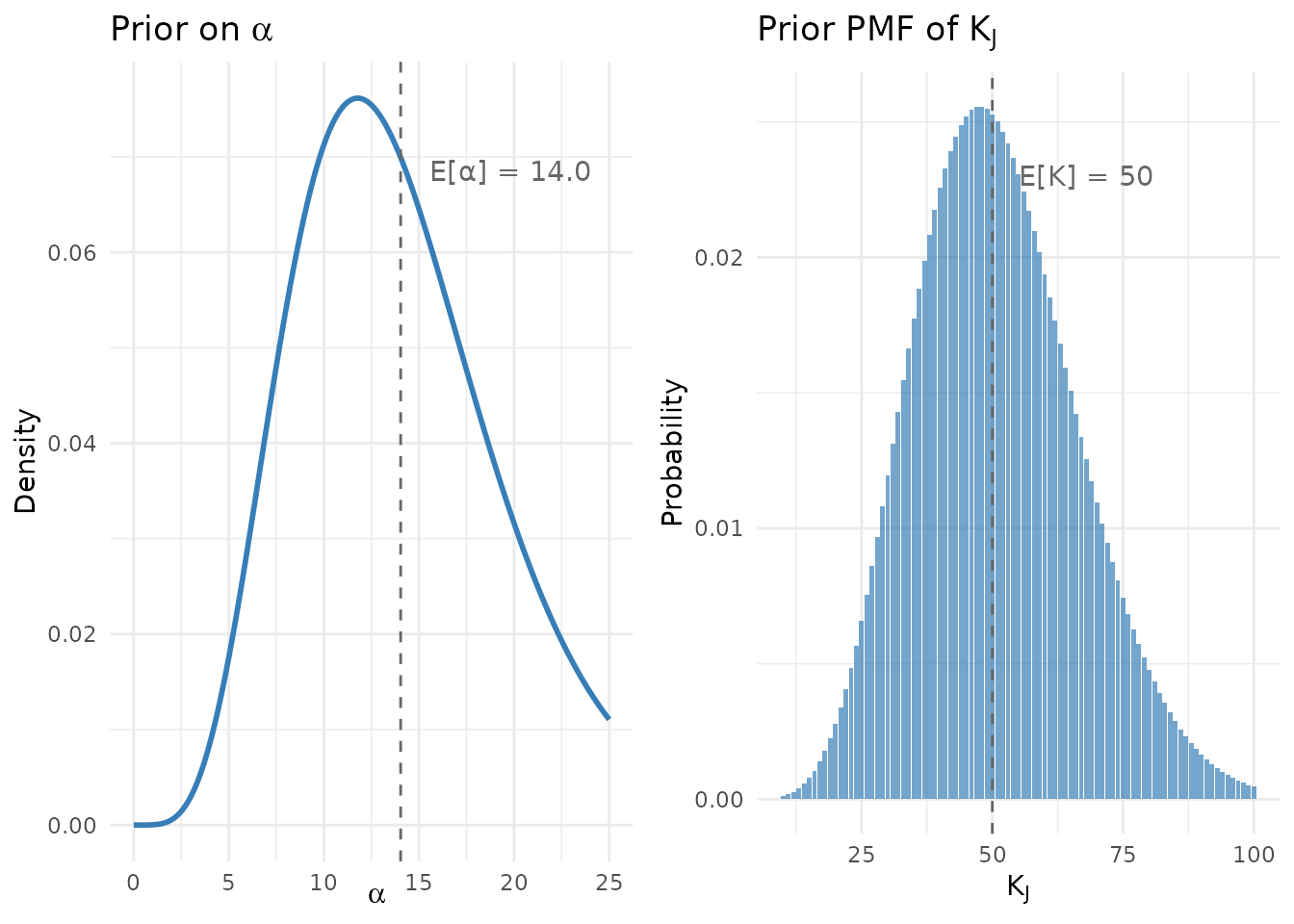

Prior distributions for the Alabama Pre-K study (J = 500, μ_K = 50).

4. Reporting Prior Elicitation in Publications

4.1 Key Elements to Report

When reporting prior elicitation in a publication, include:

1. Study context: Number of units ($J$) and their nature
2. Substantive rationale: Why you expect a certain number of clusters
3. Uncertainty characterization: Confidence level or variance specification
4. Algorithm used: A1, A2-MN, or A2-KL
5. Resulting hyperparameters: The $\text{Gamma}(a, b)$ specification
6. Diagnostic summary: Named quantities such as $P(W_{SB} > 0.5)$, separately named certified $W_{max}$ upper-bound evidence only when its typed method contract authorizes it, and the status/usable/verified/message quartet
7. Sensitivity analysis: Results for alternative specifications

Summary

This vignette demonstrated how to apply the DPprior package across three diverse research contexts:

Case Study	J	μ_K	Key Insight
CCT Multisite Trial	38	5	Dual-anchor refinement essential for low-information settings
BAI Meta-Analysis	117	18	Multiple heterogeneity sources suggest more clusters
Alabama Pre-K VAM	500	50	Large-scale applications work within package limits

Key Takeaways:

1. Context matters: The appropriate $\mu_K$ depends on substantive domain knowledge about heterogeneity sources

2. Diagnostics are essential: Always verify weight behavior, not just cluster counts

3. Dual-anchor refinement: When a named weight tail is unacceptable, use DPprior_dual_hard() for a genuine inequality or DPprior_dual_soft() for an explicit fixed-scale trade-off

4. Sensitivity analysis is mandatory: Report results across plausible alternative specifications

5. Transparent reporting: Document the complete elicitation process in publications

References

Barrera-Osorio, F., Linden, L. L., & Saavedra, J. E. (2019). Medium- and long-term educational consequences of alternative conditional cash transfer designs: Experimental evidence from Colombia. American Economic Journal: Applied Economics, 11(3), 54–91. https://doi.org/10.1257/app.20170008

Lee, J., Che, J., Rabe-Hesketh, S., Feller, A., & Miratrix, L. (2025). Improving the estimation of site-specific effects and their distribution in multisite trials. Journal of Educational and Behavioral Statistics, 50(5), 731–764. https://doi.org/10.3102/10769986241254286

Pustejovsky, J. E., & Tipton, E. (2022). Meta-analysis with robust variance estimation: Expanding the range of working models. Prevention Science, 23(3), 425–438. https://doi.org/10.1007/s11121-021-01246-3

Tanner-Smith, E. E., & Lipsey, M. W. (2015). Brief alcohol interventions for adolescents and young adults: A systematic review and meta-analysis. Journal of Substance Abuse Treatment, 51, 1–18. https://doi.org/10.1016/j.jsat.2014.09.001

---

For questions or feedback, please visit the GitHub repository.