Creates visualizations of a prior elicitation result. Multiple plot types are available, including individual distribution plots and comprehensive dashboards.
Arguments
- x
A
DPprior_fitobject.- type
Character; the type of plot to create:
- "auto"
(Default) Automatically selects the appropriate plot type. Uses
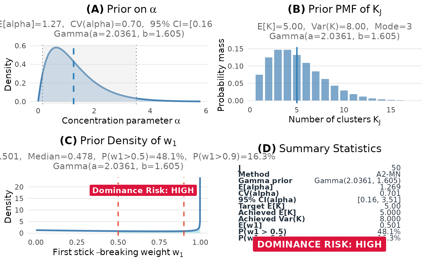
"dual"for dual-anchor fits,"dashboard"otherwise.- "dashboard"
4-panel dashboard showing alpha, K, w1, and summary.
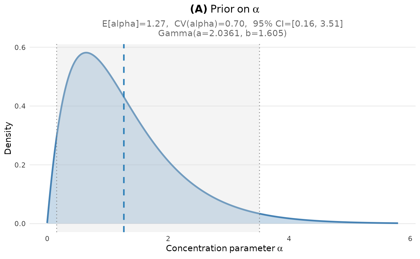
- "alpha"
Prior density of the concentration parameter alpha.
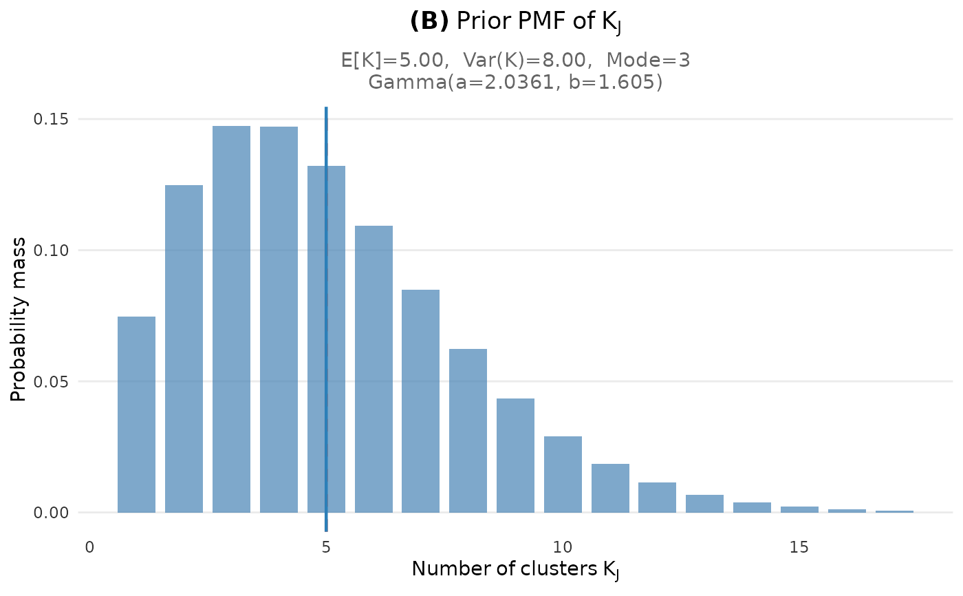
- "K"
Prior PMF of the number of clusters \(K_J\).
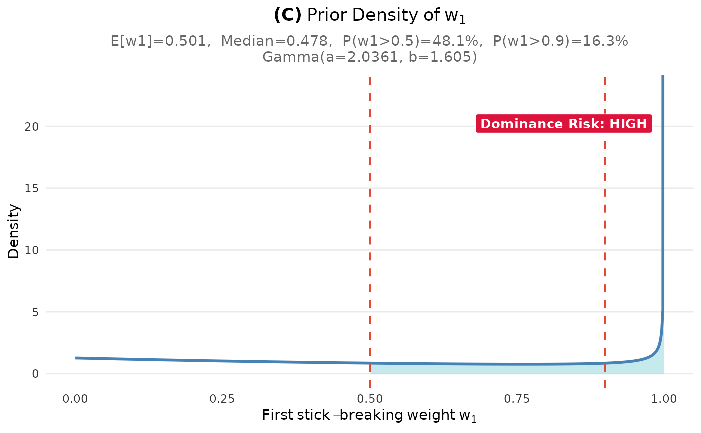
- "w1"
Prior density of the first stick-breaking weight w1.
- "dual"
Dual-anchor comparison dashboard (for dual-anchor fits).
- "comparison"
Same as "dual".
- engine
Character; graphics engine to use:
"ggplot2"(default) or"base".- ...
Additional arguments passed to the underlying plot functions. Common options include:
- base_size
Base font size (default: 11)
- ci_level
Credible interval level for alpha plot (default: 0.95)
- title
Optional title for the dashboard
- show
If TRUE, display the plot; if FALSE, return silently
Value
Depends on the plot type and engine:
For ggplot2: Returns a ggplot object or gtable (for dashboards)
For base: Returns invisible(NULL)
Details
The "auto" type is recommended for most use cases. It automatically
detects whether the fit object is from dual-anchor calibration and selects
the appropriate visualization.
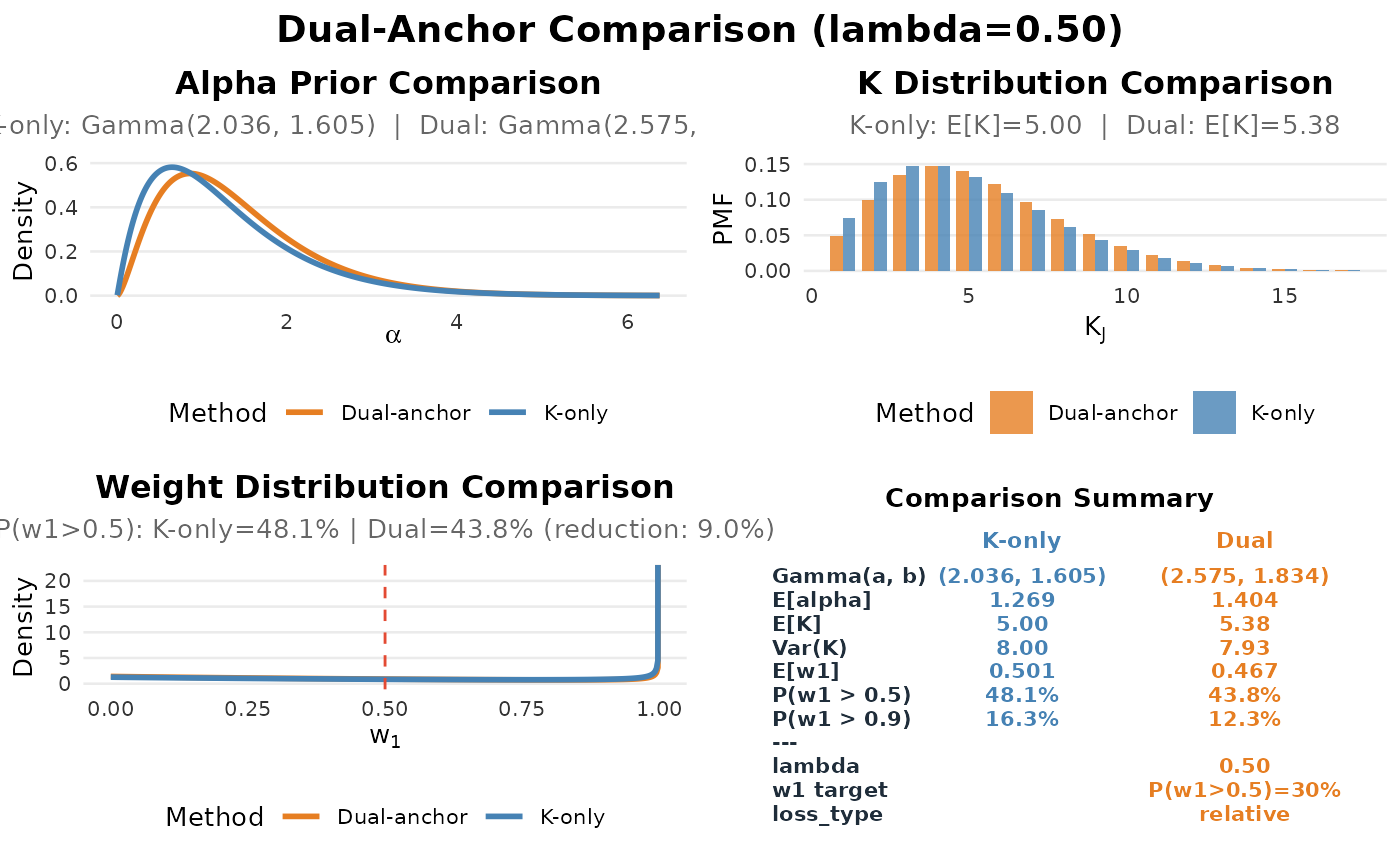
For dual-anchor fits, the comparison dashboard shows:
Alpha prior: K-only vs Dual-anchor
K distribution comparison
w1 distribution comparison with dominance threshold
Summary comparison table
Plot Type Details
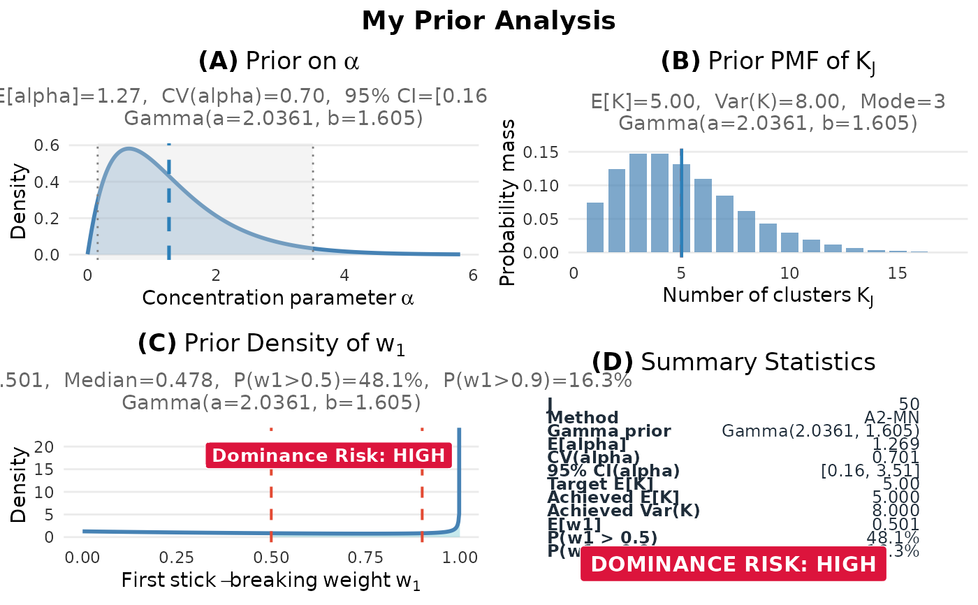
- dashboard
A 2x2 grid showing: (A) Alpha prior density with CI (B) \(K_J\) prior PMF with mode and mean (C) w1 prior density with dominance shading (D) Summary statistics table
- alpha
Gamma(a, b) density with: - Mean line (dashed) - Credible interval (shaded region) - Annotation with moments and CI
- K
Bar plot of \(P(K_J = k)\) with: - Target mean line - Achieved mean line - Optional CDF overlay
- w1
Density plot with: - Dominance region shading (w1 > 0.5) - Threshold lines - Exceedance probabilities
Examples
# Create a fit object
fit <- DPprior_fit(J = 50, mu_K = 5, var_K = 8)
#> Warning: HIGH DOMINANCE RISK: P(w1 > 0.5) = 48.1% exceeds 40%.
#> This may indicate unintended prior behavior (Lee, 2026).
#> Consider using DPprior_dual() for weight-constrained elicitation.
#> See ?DPprior_diagnostics for interpretation.
# Auto-detect best plot type
plot(fit)
 #> TableGrob (2 x 2) "dpprior_dashboard": 4 grobs
#> z cells name grob
#> 1 1 (1-1,1-1) dpprior_dashboard gtable[layout]
#> 2 2 (2-2,1-1) dpprior_dashboard gtable[layout]
#> 3 3 (1-1,2-2) dpprior_dashboard gtable[layout]
#> 4 4 (2-2,2-2) dpprior_dashboard gtable[layout]
# Specific plot types
plot(fit, type = "alpha")
#> TableGrob (2 x 2) "dpprior_dashboard": 4 grobs
#> z cells name grob
#> 1 1 (1-1,1-1) dpprior_dashboard gtable[layout]
#> 2 2 (2-2,1-1) dpprior_dashboard gtable[layout]
#> 3 3 (1-1,2-2) dpprior_dashboard gtable[layout]
#> 4 4 (2-2,2-2) dpprior_dashboard gtable[layout]
# Specific plot types
plot(fit, type = "alpha")

 plot(fit, type = "K")
 plot(fit, type = "w1")
 plot(fit, type = "dashboard")
 #> TableGrob (2 x 2) "dpprior_dashboard": 4 grobs
#> z cells name grob
#> 1 1 (1-1,1-1) dpprior_dashboard gtable[layout]
#> 2 2 (2-2,1-1) dpprior_dashboard gtable[layout]
#> 3 3 (1-1,2-2) dpprior_dashboard gtable[layout]
#> 4 4 (2-2,2-2) dpprior_dashboard gtable[layout]
# With custom options
plot(fit, type = "dashboard", title = "My Prior Analysis")
#> TableGrob (2 x 2) "dpprior_dashboard": 4 grobs
#> z cells name grob
#> 1 1 (1-1,1-1) dpprior_dashboard gtable[layout]
#> 2 2 (2-2,1-1) dpprior_dashboard gtable[layout]
#> 3 3 (1-1,2-2) dpprior_dashboard gtable[layout]
#> 4 4 (2-2,2-2) dpprior_dashboard gtable[layout]
# With custom options
plot(fit, type = "dashboard", title = "My Prior Analysis")
 #> TableGrob (3 x 2) "dpprior_dashboard": 5 grobs
#> z cells name grob
#> 1 1 (2-2,1-1) dpprior_dashboard gtable[layout]
#> 2 2 (3-3,1-1) dpprior_dashboard gtable[layout]
#> 3 3 (2-2,2-2) dpprior_dashboard gtable[layout]
#> 4 4 (3-3,2-2) dpprior_dashboard gtable[layout]
#> 5 5 (1-1,1-2) dpprior_dashboard text[GRID.text.710]
# Dual-anchor comparison
fit_K <- DPprior_a2_newton(J = 50, mu_K = 5, var_K = 8)
fit_dual <- DPprior_dual(fit_K, w1_target = list(prob = list(threshold = 0.5, value = 0.3)))
plot(fit_dual) # Auto-selects dual comparison
#> TableGrob (3 x 2) "dpprior_dashboard": 5 grobs
#> z cells name grob
#> 1 1 (2-2,1-1) dpprior_dashboard gtable[layout]
#> 2 2 (3-3,1-1) dpprior_dashboard gtable[layout]
#> 3 3 (2-2,2-2) dpprior_dashboard gtable[layout]
#> 4 4 (3-3,2-2) dpprior_dashboard gtable[layout]
#> 5 5 (1-1,1-2) dpprior_dashboard text[GRID.text.710]
# Dual-anchor comparison
fit_K <- DPprior_a2_newton(J = 50, mu_K = 5, var_K = 8)
fit_dual <- DPprior_dual(fit_K, w1_target = list(prob = list(threshold = 0.5, value = 0.3)))
plot(fit_dual) # Auto-selects dual comparison
 #> TableGrob (3 x 2) "dpprior_dashboard": 5 grobs
#> z cells name grob
#> 1 1 (2-2,1-1) dpprior_dashboard gtable[layout]
#> 2 2 (3-3,1-1) dpprior_dashboard gtable[layout]
#> 3 3 (2-2,2-2) dpprior_dashboard gtable[layout]
#> 4 4 (3-3,2-2) dpprior_dashboard gtable[layout]
#> 5 5 (1-1,1-2) dpprior_dashboard text[GRID.text.886]
plot(fit_dual, type = "comparison") # Explicit
#> TableGrob (3 x 2) "dpprior_dashboard": 5 grobs
#> z cells name grob
#> 1 1 (2-2,1-1) dpprior_dashboard gtable[layout]
#> 2 2 (3-3,1-1) dpprior_dashboard gtable[layout]
#> 3 3 (2-2,2-2) dpprior_dashboard gtable[layout]
#> 4 4 (3-3,2-2) dpprior_dashboard gtable[layout]
#> 5 5 (1-1,1-2) dpprior_dashboard text[GRID.text.886]
plot(fit_dual, type = "comparison") # Explicit
 #> TableGrob (3 x 2) "dpprior_dashboard": 5 grobs
#> z cells name grob
#> 1 1 (2-2,1-1) dpprior_dashboard gtable[layout]
#> 2 2 (3-3,1-1) dpprior_dashboard gtable[layout]
#> 3 3 (2-2,2-2) dpprior_dashboard gtable[layout]
#> 4 4 (3-3,2-2) dpprior_dashboard gtable[layout]
#> 5 5 (1-1,1-2) dpprior_dashboard text[GRID.text.1059]
#> TableGrob (3 x 2) "dpprior_dashboard": 5 grobs
#> z cells name grob
#> 1 1 (2-2,1-1) dpprior_dashboard gtable[layout]
#> 2 2 (3-3,1-1) dpprior_dashboard gtable[layout]
#> 3 3 (2-2,2-2) dpprior_dashboard gtable[layout]
#> 4 4 (3-3,2-2) dpprior_dashboard gtable[layout]
#> 5 5 (1-1,1-2) dpprior_dashboard text[GRID.text.1059]