From Poisson Proxy to NegBin: The A1 Approximation Theory

JoonHo Lee

2026-01-01

Overview

This vignette provides a rigorous mathematical treatment of the A1 closed-form approximation used in the DPprior package for Gamma hyperprior elicitation. The A1 method transforms practitioner beliefs about the number of clusters $(\mu_K, \sigma^2_K)$ into Gamma hyperparameters $(a, b)$ via a Negative Binomial moment-matching procedure.

We cover:

1. The Poisson approximation for large $J$ and its theoretical foundations
2. Scaling constant selection: $\log J$ vs harmonic vs digamma
3. The Negative Binomial gamma mixture identity
4. The A1 inverse mapping (Theorem 1)
5. Error analysis and limitations of the approximation

Throughout, we carefully distinguish between established results from the literature and novel contributions of this work.

1. The Poisson Approximation for Large J

1.1 Established Result: Poisson Convergence

The starting point for the A1 approximation is a classical result on the asymptotic distribution of $K_J | \alpha$. Recall from the Poisson-Binomial representation (see vignette("theory-overview")) that: $$K_J = \sum_{i=1}^{J} B_i, \quad B_i \sim \text{Bernoulli}\left(\frac{\alpha}{\alpha + i - 1}\right).$$

Attribution. The following Poisson convergence result is established in Arratia, Barbour, and Tavaré (2000), with the rate explicitly stated in Vicentini and Jermyn (2025, Equation 10):

Theorem (Poisson Approximation). For fixed $\alpha > 0$ and $J \to \infty$: $$d_{TV}\left(p(K_J | \alpha),\ \text{Poisson}(\mathbb{E}[K_J | \alpha])\right) = O\left(\frac{1}{\log J}\right),$$where $d_{TV}$ denotes the total variation distance.

This convergence, while sublinear, provides the conceptual foundation for using a Poisson proxy in elicitation.

1.2 The Shifted Poisson Proxy

Novel Contribution. A key insight motivating the DPprior approach is that we should apply the Poisson approximation to $K_J - 1$ rather than $K_J$ directly.

Rationale. Any unshifted Poisson approximation has an unavoidable support mismatch because $K_J \geq 1$ almost surely under the CRP (at least one cluster always exists). If $Q = \text{Poisson}(\lambda)$, then: $$d_{TV}(\mathcal{L}(K_J),\ Q) \geq \frac{1}{2}Q(0) = \frac{1}{2}e^{-\lambda}.$$

For small $\lambda$ (which occurs when the elicited $\mathbb{E}[K_J]$ is close to 1), this creates a substantial lower bound on the approximation error.

The A1 proxy (shifted): $$K_J - 1 \mid \alpha \approx \text{Poisson}(\alpha \cdot c_J),$$ or equivalently $K_J \approx 1 + \text{Poisson}(\alpha \cdot c_J)$.

This shift aligns naturally with Proposition 1 from the theory vignette, since $K_J - 1$ is a sum of $J-1$ independent Bernoulli variables ($B_1 \equiv 1$).

# Visualize the CRP probabilities
J <- 50
alpha_values <- c(0.5, 1, 2, 5)

crp_data <- do.call(rbind, lapply(alpha_values, function(a) {
  i <- 1:J
  p_new <- a / (a + i - 1)
  data.frame(
    customer = i,
    prob_new_table = p_new,
    alpha = paste0("α = ", a)
  )
}))

crp_data$alpha <- factor(crp_data$alpha, levels = paste0("α = ", alpha_values))

ggplot(crp_data, aes(x = customer, y = prob_new_table, color = alpha)) +
  geom_line(linewidth = 1) +
  scale_color_manual(values = palette_main[1:4]) +
  labs(
    x = "Customer i",
    y = expression("P(new table) = " * alpha / (alpha + i - 1)),
    title = "CRP: Probability of Starting a New Table",
    subtitle = "The expected number of tables ≈ α · log(J)"
  ) +
  theme_minimal() +
  theme(legend.position = "right")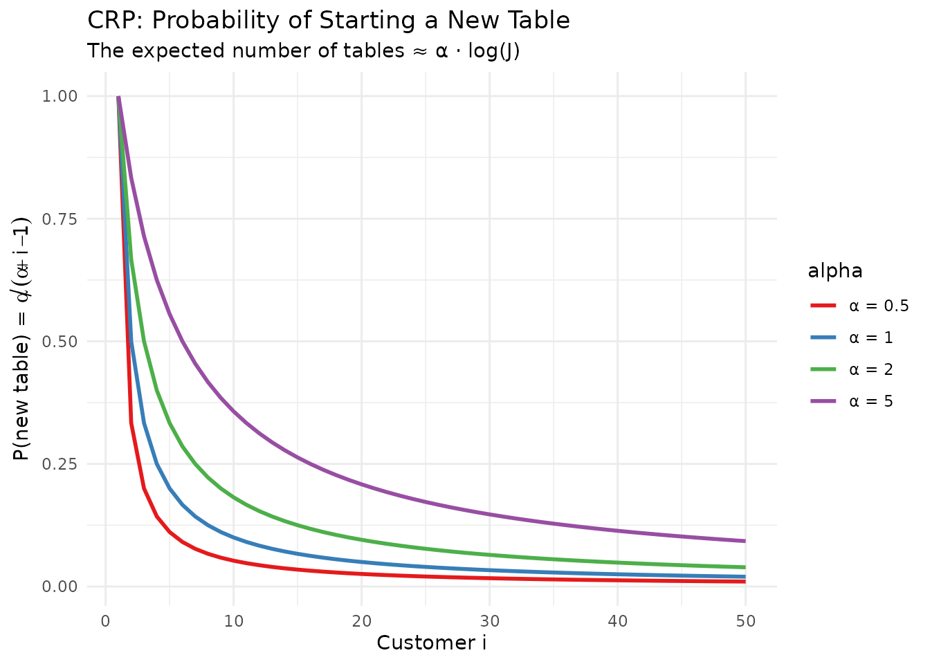

Intuition: The probability of opening a new table decreases as customers arrive.

1.3 Mean Approximation

The exact conditional mean is (see vignette("theory-overview")): $$\mu_J(\alpha) := \mathbb{E}[K_J | \alpha] = \alpha \cdot [\psi(\alpha + J) - \psi(\alpha)].$$

For the shifted mean: $$\mathbb{E}[K_J - 1 | \alpha] = \mu_J(\alpha) - 1 \approx \alpha \cdot c_J,$$ where $c_J$ is a scaling constant that we now analyze.

2. The Scaling Constant Family

2.1 Three Candidates

The A1 approximation requires a deterministic scaling constant $c_J > 0$ satisfying $\mu_J(\alpha) - 1 \approx \alpha \cdot c_J$. Three natural candidates emerge from asymptotic considerations:

Variant	Formula	Description
log (default)	$c_J = \log J$	Asymptotic leading term
harmonic	$c_J = H_{J-1} = \psi(J) + \gamma$	Better for moderate $J$
digamma	$c_J = \psi(\tilde{\alpha} + J) - \psi(\tilde{\alpha})$	Local correction

where $\gamma \approx 0.5772$ is the Euler-Mascheroni constant and $\tilde{\alpha} = (\mu_K - 1)/\log J$ is a plug-in estimate.

Lemma (Harmonic-Digamma Equivalence). For integer $J \geq 1$: $$H_{J-1} = \psi(J) + \gamma.$$

Thus, there are only two distinct mean-level competitors for integer $J$: $\log J$ and $H_{J-1}$.

# Compare scaling constants across J values
J_values <- c(10, 25, 50, 100, 200, 500)

scaling_df <- data.frame(
  J = J_values,
  log_J = sapply(J_values, function(J) compute_scaling_constant(J, "log")),
  harmonic = sapply(J_values, function(J) compute_scaling_constant(J, "harmonic"))
)

scaling_df$difference <- scaling_df$harmonic - scaling_df$log_J
scaling_df$ratio <- scaling_df$harmonic / scaling_df$log_J

knitr::kable(
  scaling_df,
  digits = 4,
  col.names = c("J", "log(J)", "H_{J-1}", "Difference", "Ratio"),
  caption = "Comparison of scaling constants"
)

Comparison of scaling constants

J	log(J)	H_{J-1}	Difference	Ratio
10	2.3026	2.8290	0.5264	1.2286
25	3.2189	3.7760	0.5571	1.1731
50	3.9120	4.4792	0.5672	1.1450
100	4.6052	5.1774	0.5722	1.1243
200	5.2983	5.8730	0.5747	1.1085
500	6.2146	6.7908	0.5762	1.0927

2.2 Asymptotic Analysis

Attribution. The following asymptotic expansion is standard (see Abramowitz & Stegun, 1964):

Proposition (Large-J Expansion). For fixed $\alpha > 0$ and $J \to \infty$: $$\mu_J(\alpha) = \alpha \log J - \alpha \psi(\alpha) + O\left(\frac{\alpha}{J}\right).$$

Moreover: $$H_{J-1} = \log J + \gamma + O\left(\frac{1}{J}\right).$$

Key insight: The “best” $\alpha$-free linear approximation $\alpha c_J$ cannot be uniform in $\alpha$ because the second-order term $-\alpha\psi(\alpha)$ depends on $\alpha$.

# Show asymptotic behavior
J <- 100
alpha_grid <- seq(0.1, 5, length.out = 100)

asymp_data <- data.frame(
  alpha = alpha_grid,
  exact = mean_K_given_alpha(J, alpha_grid),
  log_approx = alpha_grid * log(J) + 1,
  harmonic_approx = alpha_grid * (digamma(J) + 0.5772156649) + 1
)

# Reshape for plotting
asymp_long <- data.frame(
  alpha = rep(alpha_grid, 3),
  mean_K = c(asymp_data$exact, asymp_data$log_approx, asymp_data$harmonic_approx),
  Method = rep(c("Exact", "log(J) + 1", "H_{J-1} + 1"), each = length(alpha_grid))
)

asymp_long$Method <- factor(asymp_long$Method, 
                            levels = c("Exact", "log(J) + 1", "H_{J-1} + 1"))

ggplot(asymp_long, aes(x = alpha, y = mean_K, color = Method, linetype = Method)) +
  geom_line(linewidth = 1) +
  scale_color_manual(values = c("#000000", "#E41A1C", "#377EB8")) +
  scale_linetype_manual(values = c("solid", "dashed", "dotted")) +
  labs(
    x = expression(alpha),
    y = expression(E[K[J] * " | " * alpha]),
    title = expression("Exact Mean vs. Linear Approximations (J = 100)"),
    subtitle = "The approximations diverge for small and large α"
  ) +
  theme_minimal() +
  theme(legend.position = "right")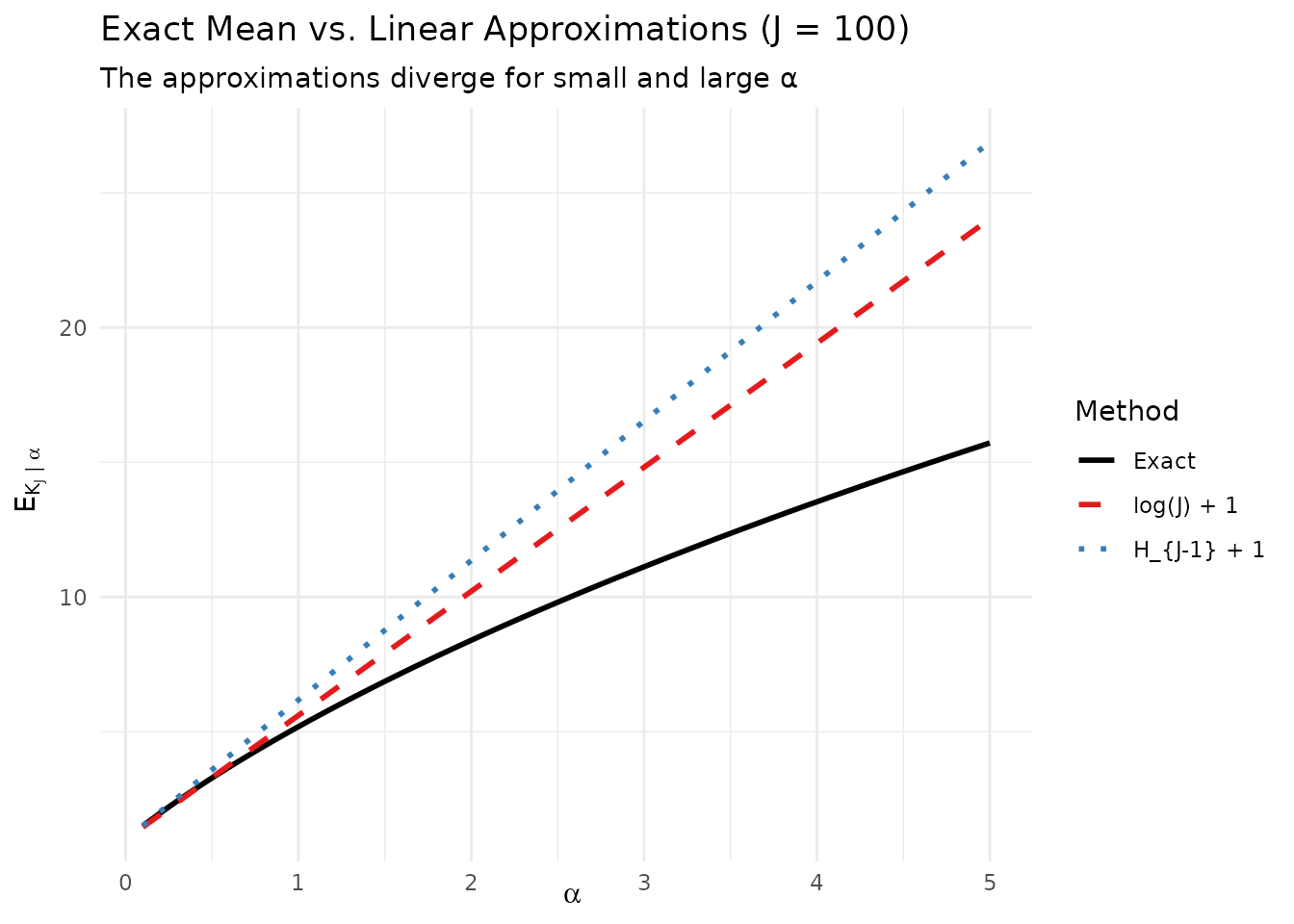

The exact mean μ_J(α) and its linear approximations.

2.3 Crossover Analysis

Novel Contribution. Define the crossover point $\alpha^*_{K-1}(J)$ as the value where the shifted mean errors are equal: $$|\mu_J(\alpha) - 1 - \alpha \log J| = |\mu_J(\alpha) - 1 - \alpha H_{J-1}|.$$

Proposition (Limiting Crossover). As $J \to \infty$: $$\alpha^*_{K-1}(J) \to x_* - 1 \approx 0.200,$$ where $x_* = \psi^{-1}(-\gamma/2) \approx 1.200$ solves $\psi(x_*) = -\gamma/2$.

Practical implication: For the shifted mean with $\alpha \gtrsim 0.2$ (which covers essentially all practical applications), the $\log J$ scaling dominates $H_{J-1}$ in terms of mean approximation error.

# Compute mean errors for different scaling choices
J_test <- 50
alpha_grid <- seq(0.1, 3, by = 0.1)

error_df <- data.frame(
  alpha = alpha_grid,
  error_log = abs(mean_K_given_alpha(J_test, alpha_grid) - 1 - 
                  alpha_grid * compute_scaling_constant(J_test, "log")),
  error_harmonic = abs(mean_K_given_alpha(J_test, alpha_grid) - 1 - 
                       alpha_grid * compute_scaling_constant(J_test, "harmonic"))
)

error_df$better <- ifelse(error_df$error_log < error_df$error_harmonic, 
                          "log(J)", "H_{J-1}")

cat("Mean error comparison for J =", J_test, "\n")
#> Mean error comparison for J = 50
cat("α range where log(J) is better:", 
    sum(error_df$better == "log(J)"), "out of", nrow(error_df), "values\n")
#> α range where log(J) is better: 29 out of 30 values
cat("Crossover occurs near α ≈", 
    error_df$alpha[which.min(abs(error_df$error_log - error_df$error_harmonic))], "\n")
#> Crossover occurs near α ≈ 0.2

2.4 Default Recommendation

Novel Contribution. Based on the crossover analysis:

Default: Use shifted Poisson with $c_J = \log J$ for the A1 approximation.

This choice:

1. Is simpler to compute
2. Provides better mean accuracy for $\alpha \gtrsim 0.2$
3. Aligns with the asymptotic leading term

3. The NegBin Gamma Mixture

3.1 The Key Identity

Attribution. The following is a standard result in Bayesian statistics (see, e.g., the Gamma-Poisson conjugacy):

Proposition (Gamma-Poisson Mixture). If $X | \lambda \sim \text{Poisson}(\lambda)$ and $\lambda \sim \text{Gamma}(a, b/(b+1))$, then: $$X \sim \text{NegBin}(a, b/(b+1)).$$

More generally, if $X | \lambda \sim \text{Poisson}(c \cdot \lambda)$ and $\lambda \sim \text{Gamma}(a, b)$, then: $$X \sim \text{NegBin}\left(a, \frac{b}{b + c}\right).$$

3.2 Application to $K_J$

Novel Application. Applying this to the A1 proxy with $\alpha \sim \text{Gamma}(a, b)$:

$$K_J - 1 \mid \alpha \approx \text{Poisson}(\alpha \cdot c_J) \quad \Longrightarrow \quad K_J - 1 \approx \text{NegBin}\left(a, \frac{b}{b + c_J}\right).$$

Under the NegBin$(r, p)$ parameterization where $p$ is the success probability:

Quantity	Formula
Mean of $K_J - 1$	$\displaystyle\frac{a \cdot c_J}{b}$
Variance of $K_J - 1$	$\displaystyle\frac{a \cdot c_J \cdot (b + c_J)}{b^2}$
Mean of $K_J$	$\displaystyle 1 + \frac{a \cdot c_J}{b}$
Variance of $K_J$	$\displaystyle\frac{a \cdot c_J \cdot (b + c_J)}{b^2}$

# Compare NegBin approximation to exact marginal
J <- 50
a <- 1.5
b <- 0.5
logS <- compute_log_stirling(J)

# Exact marginal PMF
pmf_exact <- pmf_K_marginal(J, a, b, logS)

# NegBin approximation
c_J <- log(J)
p_nb <- b / (b + c_J)

# NegBin PMF for K-1, then shift
k_vals <- 0:J
pmf_negbin <- dnbinom(k_vals - 1, size = a, prob = p_nb)
pmf_negbin[1] <- 0  # K >= 1

# Normalize for comparison
pmf_negbin <- pmf_negbin / sum(pmf_negbin)

# Create comparison data
k_show <- 1:25
comparison_df <- data.frame(
  K = rep(k_show, 2),
  Probability = c(pmf_exact[k_show + 1], pmf_negbin[k_show + 1]),
  Method = rep(c("Exact Marginal", "NegBin Approximation"), each = length(k_show))
)

ggplot(comparison_df, aes(x = K, y = Probability, fill = Method)) +
  geom_bar(stat = "identity", position = "dodge", alpha = 0.8) +
  scale_fill_manual(values = c("#377EB8", "#E41A1C")) +
  labs(
    x = expression(K[J]),
    y = "Probability",
    title = expression("NegBin Approximation vs Exact Marginal (J = 50)"),
    subtitle = paste0("Gamma(", a, ", ", b, ") prior on α")
  ) +
  theme_minimal() +
  theme(legend.position = "bottom")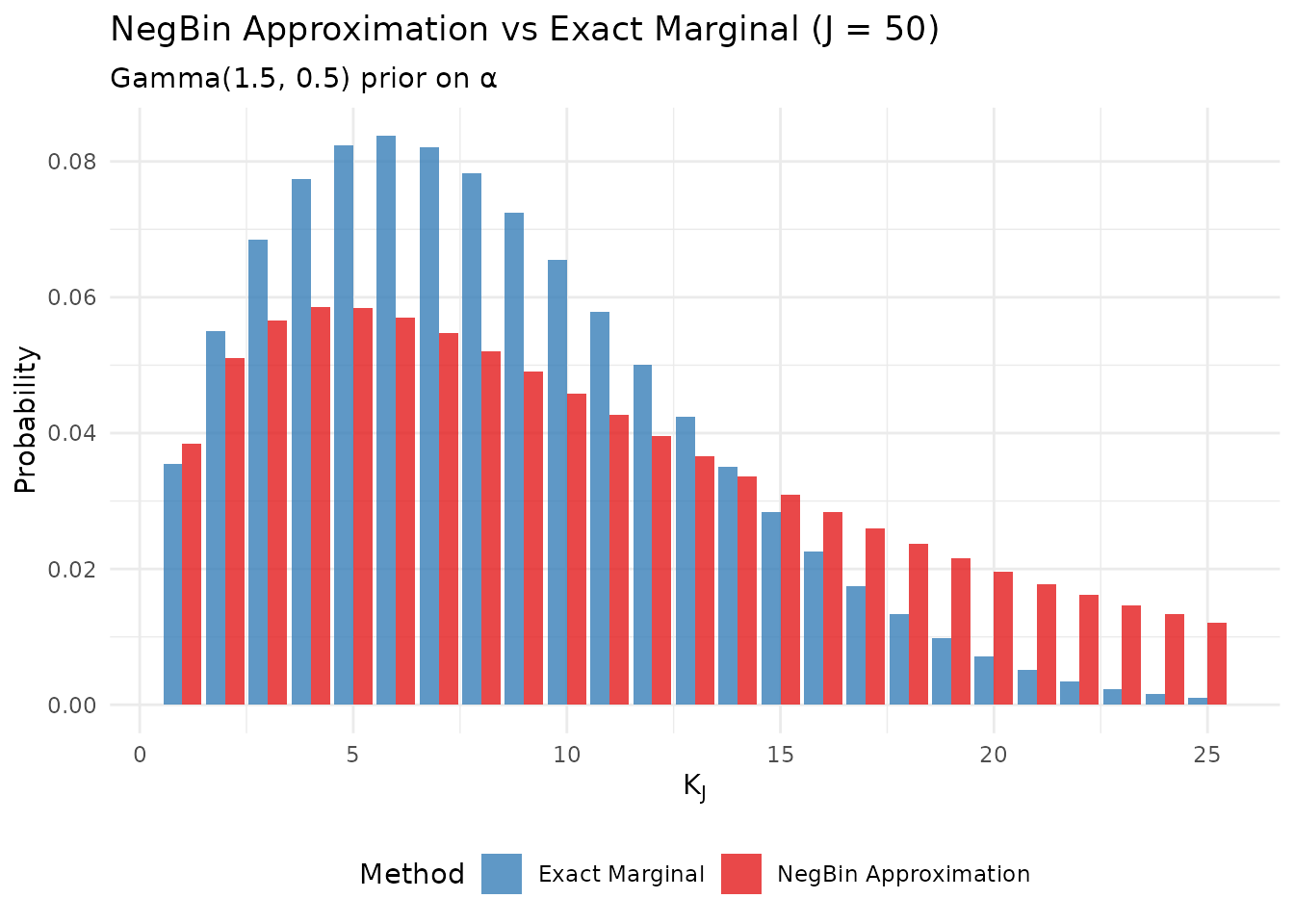

The NegBin approximation vs exact marginal distribution.

4. The A1 Inverse Mapping (Theorem 1)

4.1 The Inverse Problem

Given practitioner-specified beliefs $(\mu_K, \sigma^2_K)$ about the number of clusters, we seek the Gamma hyperparameters $(a, b)$ such that the marginal distribution of $K_J$ has the desired moments.

Under the NegBin proxy, this becomes a moment-matching problem with an analytical solution.

4.2 Main Result

Novel Contribution. The following theorem provides the closed-form inverse mapping that is central to the A1 method:

Theorem 1 (A1 Inverse Mapping). Fix $J \geq 2$ and scaling constant $c_J > 0$. Define the shifted mean $m := \mu_K - 1$.

If $m > 0$ and $\sigma^2_K > m$ (overdispersion), then there exists a unique $(a, b) \in (0, \infty)^2$ that matches $(\mu_K, \sigma^2_K)$ under the NegBin proxy, given by: $$\boxed{ a = \frac{m^2}{\sigma^2_K - m}, \qquad b = \frac{m \cdot c_J}{\sigma^2_K - m} }$$

Proof. From the NegBin moments: $$\mu_K = 1 + \frac{a \cdot c_J}{b} \quad \Rightarrow \quad b = \frac{a \cdot c_J}{m}.$$

Substituting into the variance equation $\sigma^2_K = \frac{a \cdot c_J \cdot (b + c_J)}{b^2}$: $$\sigma^2_K = \frac{a \cdot c_J \cdot (b + c_J)}{b^2} = m + \frac{m^2}{a}.$$

Solving for $a$: $$a = \frac{m^2}{\sigma^2_K - m}.$$

Positivity requires $\sigma^2_K > m$, which is the overdispersion condition. $\square$

4.3 Corollary: Interpretation for $\alpha$

Corollary 1. Under Theorem 1: $$\mathbb{E}[\alpha] = \frac{a}{b} = \frac{m}{c_J}, \qquad \text{Var}(\alpha) = \frac{a}{b^2} = \frac{\sigma^2_K - m}{c_J^2}, \qquad \text{CV}(\alpha) = \frac{1}{\sqrt{a}} = \frac{\sqrt{\sigma^2_K - m}}{m}.$$

Interpretation: Under A1, $\mu_K$ determines the prior mean of $\alpha$, while the “confidence” (through $\sigma^2_K - m$) determines the prior variance of $\alpha$.

# Demonstrate the A1 mapping
J <- 50
mu_K <- 5
var_K <- 8

# Step-by-step calculation
m <- mu_K - 1
D <- var_K - m
c_J <- log(J)

cat("A1 Inverse Mapping Demonstration\n")
#> A1 Inverse Mapping Demonstration
cat(paste(rep("=", 50), collapse = ""), "\n\n")
#> ==================================================

cat("Inputs:\n")
#> Inputs:
cat(sprintf("  J = %d\n", J))
#>   J = 50
cat(sprintf("  μ_K = %.1f\n", mu_K))
#>   μ_K = 5.0
cat(sprintf("  σ²_K = %.1f\n\n", var_K))
#>   σ²_K = 8.0

cat("Intermediate calculations:\n")
#> Intermediate calculations:
cat(sprintf("  m = μ_K - 1 = %.1f\n", m))
#>   m = μ_K - 1 = 4.0
cat(sprintf("  D = σ²_K - m = %.1f\n", D))
#>   D = σ²_K - m = 4.0
cat(sprintf("  c_J = log(J) = %.4f\n\n", c_J))
#>   c_J = log(J) = 3.9120

cat("A1 formulas:\n")
#> A1 formulas:
cat(sprintf("  a = m² / D = %.1f² / %.1f = %.4f\n", m, D, m^2/D))
#>   a = m² / D = 4.0² / 4.0 = 4.0000
cat(sprintf("  b = m · c_J / D = %.1f × %.4f / %.1f = %.4f\n\n", m, c_J, D, m*c_J/D))
#>   b = m · c_J / D = 4.0 × 3.9120 / 4.0 = 3.9120

# Use DPprior_a1 to verify
fit <- DPprior_a1(J = J, mu_K = mu_K, var_K = var_K)

cat("DPprior_a1() result:\n")
#> DPprior_a1() result:
cat(sprintf("  a = %.4f\n", fit$a))
#>   a = 4.0000
cat(sprintf("  b = %.4f\n", fit$b))
#>   b = 3.9120
cat(sprintf("  E[α] = a/b = %.4f\n", fit$a / fit$b))
#>   E[α] = a/b = 1.0225
cat(sprintf("  CV(α) = 1/√a = %.4f\n", 1/sqrt(fit$a)))
#>   CV(α) = 1/√a = 0.5000

4.4 Feasibility Region

Novel Contribution. The feasibility constraints for A1 are:

Shifted A1 (default, for DP partitions): $$\mu_K > 1 \quad \text{and} \quad \sigma^2_K > \mu_K - 1.$$

These are proxy-model constraints arising from the NegBin moment identity, not fundamental constraints of the DP itself.

Important: Some user specifications with $\sigma^2_K \leq \mu_K - 1$ may be feasible under the exact DP but infeasible under A1. In such cases, the package projects to the feasibility boundary.

# Demonstrate feasibility projection
cat("Feasibility Demonstration\n")
#> Feasibility Demonstration
cat(paste(rep("=", 50), collapse = ""), "\n\n")
#> ==================================================

# Case 1: Feasible
fit1 <- DPprior_a1(J = 50, mu_K = 5, var_K = 8)
cat("Case 1: Feasible (var_K = 8 > μ_K - 1 = 4)\n")
#> Case 1: Feasible (var_K = 8 > μ_K - 1 = 4)
cat(sprintf("  Status: %s\n\n", fit1$status))
#>   Status: success

# Case 2: Infeasible - requires projection
fit2 <- DPprior_a1(J = 50, mu_K = 5, var_K = 3)
#> Warning: var_K <= mu_K - 1: projected to feasible boundary
cat("Case 2: Infeasible (var_K = 3 < μ_K - 1 = 4)\n")
#> Case 2: Infeasible (var_K = 3 < μ_K - 1 = 4)
cat(sprintf("  Status: %s\n", fit2$status))
#>   Status: projected
cat(sprintf("  Original var_K: %.1f\n", 3))
#>   Original var_K: 3.0
cat(sprintf("  Projected var_K: %.6f\n", fit2$target$var_K_used))

4.5 Near-Boundary Sensitivity

Novel Contribution. Define $D := \sigma^2_K - m$. As $D \downarrow 0$: $$a \sim \frac{m^2}{D} \to \infty, \qquad b \sim \frac{m \cdot c_J}{D} \to \infty,$$ while $\mathbb{E}[\alpha] = m/c_J$ remains finite.

The sensitivities scale as $O(D^{-2})$, meaning that high-confidence specifications (small $D$) lead to numerically ill-conditioned mappings. This motivates the projection buffer in the implementation.

5. Error Analysis

5.1 Sources of Approximation Error

The A1 method introduces several sources of error:

1. Poisson proxy error: The finite-$J$ deviation from the Poisson limit
2. Scaling constant choice: Different $c_J$ options introduce different biases
3. Moment matching vs. distribution matching: Even if moments match, the full distributions may differ

5.2 Quantifying Moment Error

Novel Contribution. We can directly compare the A1-achieved moments against the exact marginal moments:

# Compare A1 moments to exact moments
test_cases <- expand.grid(
  J = c(25, 50, 100, 200),
  mu_K = c(5, 10),
  vif = c(1.5, 2, 3)
)

# Filter valid cases first
test_cases <- test_cases[test_cases$mu_K < test_cases$J, ]

results <- do.call(rbind, lapply(1:nrow(test_cases), function(i) {
  J <- test_cases$J[i]
  mu_K <- test_cases$mu_K[i]
  vif <- test_cases$vif[i]
  var_K <- vif * (mu_K - 1)
  
  # A1 mapping
  fit <- DPprior_a1(J = J, mu_K = mu_K, var_K = var_K)
  
  # Exact moments with A1 parameters
  exact <- exact_K_moments(J, fit$a, fit$b)
  
  data.frame(
    J = J,
    mu_K_target = mu_K,
    var_K_target = var_K,
    mu_K_achieved = exact$mean,
    var_K_achieved = exact$var,
    mu_error_pct = 100 * (exact$mean - mu_K) / mu_K,
    var_error_pct = 100 * (exact$var - var_K) / var_K
  )
}))

knitr::kable(
  results,
  digits = c(0, 1, 1, 2, 2, 1, 1),
  col.names = c("J", "μ_K (target)", "σ²_K (target)", 
                "μ_K (achieved)", "σ²_K (achieved)",
                "Mean Error %", "Var Error %"),
  caption = "A1 approximation error: target vs. achieved moments"
)

A1 approximation error: target vs. achieved moments

J	μ_K (target)	σ²_K (target)	μ_K (achieved)	σ²_K (achieved)	Mean Error %	Var Error %
25	5	6.0	4.27	3.22	-14.6	-46.3
50	5	6.0	4.51	3.89	-9.8	-35.2
100	5	6.0	4.67	4.37	-6.6	-27.2
200	5	6.0	4.77	4.72	-4.5	-21.3
25	10	13.5	6.84	4.58	-31.6	-66.0
50	10	13.5	7.64	6.21	-23.6	-54.0
100	10	13.5	8.21	7.53	-17.9	-44.2
200	10	13.5	8.61	8.57	-13.9	-36.5
25	5	8.0	4.21	3.86	-15.8	-51.7
50	5	8.0	4.46	4.78	-10.8	-40.2
100	5	8.0	4.63	5.48	-7.5	-31.5
200	5	8.0	4.74	6.00	-5.2	-25.0
25	10	18.0	6.78	5.31	-32.2	-70.5
50	10	18.0	7.59	7.43	-24.1	-58.7
100	10	18.0	8.16	9.24	-18.4	-48.7
200	10	18.0	8.57	10.70	-14.3	-40.6
25	5	12.0	4.10	4.98	-17.9	-58.5
50	5	12.0	4.37	6.40	-12.6	-46.7
100	5	12.0	4.55	7.52	-9.0	-37.4
200	5	12.0	4.67	8.38	-6.6	-30.2
25	10	27.0	6.67	6.67	-33.3	-75.3
50	10	27.0	7.48	9.76	-25.2	-63.8
100	10	27.0	8.07	12.51	-19.3	-53.7
200	10	27.0	8.49	14.79	-15.1	-45.2

5.3 Systematic Patterns

# Create heatmap of A1 mean errors
J_grid <- c(20, 30, 50, 75, 100, 150, 200)
mu_grid <- seq(3, 15, by = 2)

error_matrix <- matrix(NA, nrow = length(J_grid), ncol = length(mu_grid))
rownames(error_matrix) <- paste0("J=", J_grid)
colnames(error_matrix) <- paste0("μ=", mu_grid)

for (i in seq_along(J_grid)) {
  for (j in seq_along(mu_grid)) {
    J <- J_grid[i]
    mu_K <- mu_grid[j]
    
    if (mu_K < J) {
      var_K <- 2 * (mu_K - 1)  # VIF = 2
      fit <- DPprior_a1(J = J, mu_K = mu_K, var_K = var_K)
      exact <- exact_K_moments(J, fit$a, fit$b)
      error_matrix[i, j] <- 100 * (exact$mean - mu_K) / mu_K
    }
  }
}

# Convert to data frame for ggplot
error_df <- expand.grid(J = J_grid, mu_K = mu_grid)
error_df$error <- as.vector(error_matrix)

ggplot(error_df[!is.na(error_df$error), ], 
       aes(x = factor(mu_K), y = factor(J), fill = error)) +
  geom_tile() +
  geom_text(aes(label = sprintf("%.1f%%", error)), color = "white", size = 3) +
  scale_fill_gradient2(low = "#377EB8", mid = "white", high = "#E41A1C",
                       midpoint = 0, name = "Mean\nError %") +
  labs(
    x = expression("Target " * mu[K]),
    y = "Sample Size J",
    title = "A1 Mean Error Pattern",
    subtitle = "VIF = 2 for all cases"
  ) +
  theme_minimal()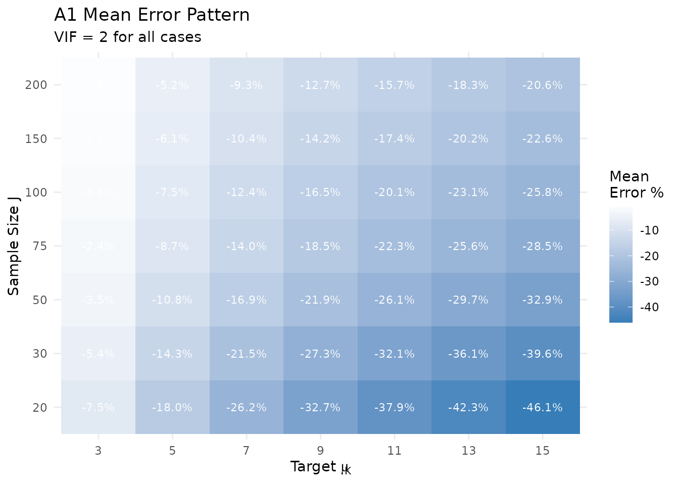

A1 mean error as a function of J and μ_K.

5.4 Critical Warning: NegBin Marginal Limitations

Novel Finding. Tables from the research notes demonstrate that the NegBin marginal approximation can produce:

• Mean errors of 40-75%
• Variance errors of 230-730%

This confirms that A1 should be viewed primarily as an initializer, not as a final solution. The A2 Newton refinement (see vignette("theory-newton")) should be applied for any application requiring accurate moment matching.

# Compare A1 to A2 refinement
J <- 50
mu_K <- 5
var_K <- 8

# A1 only
fit_a1 <- DPprior_a1(J = J, mu_K = mu_K, var_K = var_K)
exact_a1 <- exact_K_moments(J, fit_a1$a, fit_a1$b)

# A2 refinement (full DPprior_fit)
fit_a2 <- DPprior_fit(J = J, mu_K = mu_K, var_K = var_K)
#> Warning: HIGH DOMINANCE RISK: P(w1 > 0.5) = 48.1% exceeds 40%.
#>   This may indicate unintended prior behavior (RN-07).
#>   Consider using DPprior_dual() for weight-constrained elicitation.
#>   See ?DPprior_diagnostics for interpretation.
exact_a2 <- exact_K_moments(J, fit_a2$a, fit_a2$b)

cat("Comparison: A1 vs A2 Refinement\n")
#> Comparison: A1 vs A2 Refinement
cat(paste(rep("=", 50), collapse = ""), "\n\n")
#> ==================================================

cat(sprintf("Target: μ_K = %.1f, σ²_K = %.1f\n\n", mu_K, var_K))
#> Target: μ_K = 5.0, σ²_K = 8.0

cat("A1 (closed-form):\n")
#> A1 (closed-form):
cat(sprintf("  Parameters: a = %.4f, b = %.4f\n", fit_a1$a, fit_a1$b))
#>   Parameters: a = 4.0000, b = 3.9120
cat(sprintf("  Achieved:   μ_K = %.4f, σ²_K = %.4f\n", exact_a1$mean, exact_a1$var))
#>   Achieved:   μ_K = 4.4614, σ²_K = 4.7831
cat(sprintf("  Errors:     %.2f%% (mean), %.2f%% (var)\n\n",
            100 * (exact_a1$mean - mu_K) / mu_K,
            100 * (exact_a1$var - var_K) / var_K))
#>   Errors:     -10.77% (mean), -40.21% (var)

cat("A2 (Newton refinement):\n")
#> A2 (Newton refinement):
cat(sprintf("  Parameters: a = %.4f, b = %.4f\n", fit_a2$a, fit_a2$b))
#>   Parameters: a = 2.0361, b = 1.6051
cat(sprintf("  Achieved:   μ_K = %.6f, σ²_K = %.6f\n", exact_a2$mean, exact_a2$var))
#>   Achieved:   μ_K = 5.000000, σ²_K = 8.000000
cat(sprintf("  Errors:     %.2e%% (mean), %.2e%% (var)\n",
            100 * abs(exact_a2$mean - mu_K) / mu_K,
            100 * abs(exact_a2$var - var_K) / var_K))
#>   Errors:     1.66e-08% (mean), 9.44e-08% (var)

6. Summary

This vignette has provided a rigorous treatment of the A1 approximation theory:

1. Poisson approximation: The classical result that $K_J - 1 | \alpha$ converges to Poisson$(\alpha \cdot c_J)$ provides the theoretical foundation.

2. Scaling constant: The default $c_J = \log J$ provides the best mean-level accuracy for typical $\alpha$ values.

3. NegBin mixture: When $\alpha \sim \text{Gamma}(a, b)$, the marginal $K_J - 1$ approximately follows a Negative Binomial distribution.

4. Inverse mapping: Theorem 1 provides closed-form expressions for $(a, b)$ given target moments $(\mu_K, \sigma^2_K)$.

5. Limitations: The A1 approximation can have substantial errors and should be viewed as an initializer for the A2 Newton refinement.

References

Abramowitz, M., & Stegun, I. A. (1964). Handbook of Mathematical Functions. National Bureau of Standards.

Antoniak, C. E. (1974). Mixtures of Dirichlet processes with applications to Bayesian nonparametric problems. The Annals of Statistics, 2(6), 1152-1174.

Arratia, R., Barbour, A. D., & Tavaré, S. (2000). The number of components in a logarithmic combinatorial structure. The Annals of Applied Probability, 10(2), 331-361.

Dorazio, R. M. (2009). On selecting a prior for the precision parameter of Dirichlet process mixture models. Journal of Statistical Planning and Inference, 139(10), 3384-3390.

Murugiah, S., & Sweeting, T. J. (2012). Selecting the precision parameter prior in Dirichlet process mixture models. Journal of Statistical Computation and Simulation, 82(9), 1307-1322.

Vicentini, C., & Jermyn, I. H. (2025). Prior selection for the precision parameter of Dirichlet process mixtures. arXiv:2502.00864.

---

For questions about this vignette or the DPprior package, please visit the GitHub repository.