DPprior: Why Prior Elicitation Matters

JoonHo Lee

2026-01-01

Introduction

The DPprior package provides tools for principled prior elicitation on the concentration parameter $\alpha$ in Dirichlet Process (DP) mixture models. Rather than requiring researchers to think directly in terms of the abstract parameter $\alpha$, DPprior allows specification through two intuitive dimensions: expected cluster counts—how many distinct groups do you anticipate?—and cluster weight concentration—how evenly do you expect observations to be distributed across those groups? These are quantities that applied researchers can often reason about based on domain knowledge, and DPprior translates such beliefs into principled Gamma hyperpriors on $\alpha$.

Installation

# From CRAN (when available)
install.packages("DPprior")

# From GitHub (development version)
devtools::install_github("joonho112/DPprior")

library(DPprior)

The Core Problem

When using DP mixture models for applications such as multisite trials, meta-analysis, or Bayesian nonparametric density estimation, researchers must specify a prior on the concentration parameter $\alpha$. This parameter governs the model’s clustering behavior, affecting multiple dimensions:

• How many clusters will the model tend to produce?
• How are observations distributed across clusters—evenly, or with one dominant group?
• How much shrinkage will the posterior exhibit toward a common mean?

In low-information settings—where the number of observations $J$ is moderate (e.g., 25–100) and per-observation information is limited—the prior on $\alpha$ can substantially influence posterior inference. The DPprior package addresses the critical question: How should researchers translate their domain knowledge into a principled prior on $\alpha$?

The Core Challenge: Why $\alpha$ Matters

The Dirichlet Process Mixture Model

In a DP mixture model, we place a Dirichlet Process prior on an unknown distribution $G$: $$G \sim \text{DP}(\alpha, G_0),$$ where $G_0$ is the base (centering) measure and $\alpha > 0$ is the concentration parameter. Observations $\theta_1, \ldots, \theta_J$ are then drawn from $G$: $$\theta_j \mid G \stackrel{iid}{\sim} G.$$

A fundamental property of the DP is that draws from $G$ exhibit clustering: multiple observations can share the same value, with the number of distinct values $K_J$ depending critically on $\alpha$. This clustering behavior makes the DP particularly useful for applications where the number of underlying groups is unknown—such as identifying distinct treatment effect patterns across sites in a multisite trial, or discovering latent subpopulations in meta-analysis.

What Does $\alpha$ Control?

The concentration parameter $\alpha$ influences the model’s behavior in three interconnected ways:

1. Number of clusters ($K_J$): Larger $\alpha$ leads to more clusters on average; smaller $\alpha$ concentrates mass on fewer clusters. Specifically, $\mathbb{E}[K_J | \alpha] \approx \alpha \log J$ for large $J$ (Antoniak, 1974).

2. Stick-breaking weights: In Sethuraman’s (1994) representation, $G$ is constructed via stick-breaking weights $(w_1, w_2, \ldots)$ where $w_h = v_h \prod_{\ell < h}(1 - v_\ell)$ with $v_h \sim \text{Beta}(1, \alpha)$. Smaller $\alpha$ produces weights concentrated on early atoms (one or two clusters dominate); larger $\alpha$ spreads weights more evenly across many clusters. As Vicentini & Jermyn (2025) emphasize, these weights represent asymptotic relative cluster sizes and are a fundamental quantity distinct from the cluster count.

3. Posterior shrinkage: The prior on $\alpha$ affects how much the posterior borrows strength across observations. In multisite trials, this determines the degree of shrinkage toward a common mean—a key consideration when sites have varying sample sizes or precision (Lee et al., 2025).

The figure below illustrates how different values of $\alpha$ lead to dramatically different partition structures.

# Simulate stick-breaking for different alpha values
n_atoms <- 15
alpha_values <- c(0.5, 2, 10)

set.seed(123)
sb_data <- do.call(rbind, lapply(alpha_values, function(a) {
  # Simulate stick-breaking
  v <- rbeta(n_atoms, 1, a)
  w <- numeric(n_atoms)
  w[1] <- v[1]
  for (h in 2:n_atoms) {
    w[h] <- v[h] * prod(1 - v[1:(h-1)])
  }
  data.frame(
    atom = 1:n_atoms,
    weight = w,
    alpha = paste0("α = ", a)
  )
}))

sb_data$alpha <- factor(sb_data$alpha, 
                        levels = paste0("α = ", alpha_values))

ggplot(sb_data, aes(x = atom, y = weight, fill = alpha)) +
  geom_bar(stat = "identity") +
  facet_wrap(~alpha, nrow = 1) +
  scale_fill_manual(values = palette_main[1:3]) +
  labs(x = "Atom Index", 
       y = "Stick-Breaking Weight",
       title = "Effect of α on Cluster Weight Distribution",
       subtitle = "One realization from GEM(α) for each value") +
  theme_minimal() +
  theme(legend.position = "none",
        strip.text = element_text(face = "bold", size = 12))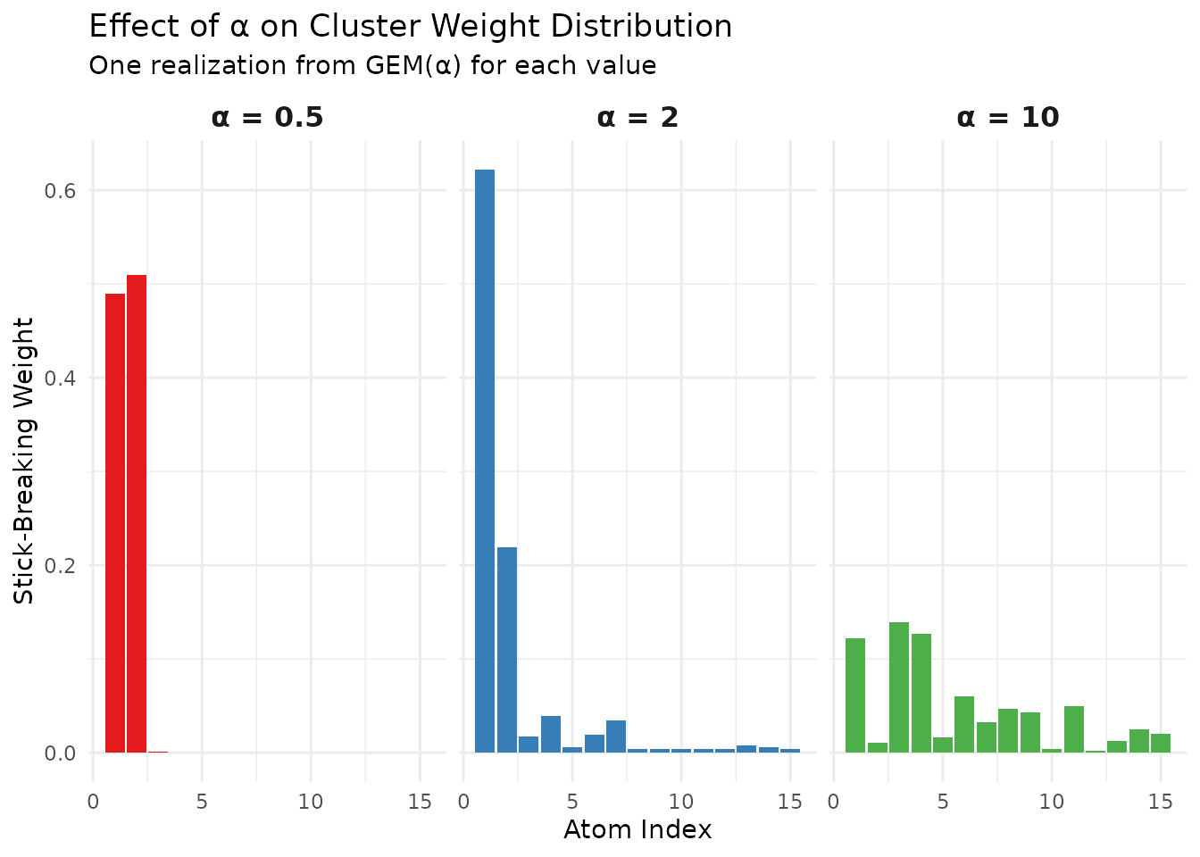

Illustration of stick-breaking weights for different values of α. Smaller α concentrates mass on the first few atoms, while larger α spreads weights more evenly.

The Distribution of $K_J$

Given $\alpha$, the number of distinct clusters $K_J$ among $J$ observations follows the Antoniak distribution (Antoniak, 1974). The probability mass function is: $$P(K_J = k | \alpha) = \frac{|s(J,k)| \cdot \alpha^k}{(\alpha)_J},$$ where $|s(J,k)|$ are unsigned Stirling numbers of the first kind and $(\alpha)_J = \alpha(\alpha+1)\cdots(\alpha+J-1)$ is the rising factorial. The expectation is: $$\mathbb{E}[K_J \mid \alpha] = \sum_{i=1}^{J} \frac{\alpha}{\alpha + i - 1} \approx \alpha \log J \quad \text{(for large } J\text{)}.$$

This relationship provides the foundation for DPprior’s elicitation approach: if a researcher can express beliefs about $K_J$, we can back out an appropriate prior on $\alpha$.

Importantly, Zito et al. (2024) showed that when $\alpha$ is random with a Gamma prior, the marginal distribution of $K_J$ converges to a Negative Binomial as $J \to \infty$. This theoretical result—which the DPprior package exploits for closed-form initial solutions—explains why randomizing $\alpha$ leads to more robust clustering behavior compared to fixing it.

# Demonstrate E[K] vs alpha relationship
alpha_grid <- seq(0.1, 5, by = 0.1)
J_values <- c(25, 50, 100)

k_data <- do.call(rbind, lapply(J_values, function(J) {
  EK <- sapply(alpha_grid, function(a) mean_K_given_alpha(J, a))
  data.frame(alpha = alpha_grid, E_K = EK, J = paste0("J = ", J))
}))

k_data$J <- factor(k_data$J, levels = paste0("J = ", J_values))

ggplot(k_data, aes(x = alpha, y = E_K, color = J)) +
  geom_line(linewidth = 1.2) +
  scale_color_manual(values = palette_main[1:3]) +
  labs(x = expression(alpha), 
       y = expression(E*"["*K[J]*"|"*alpha*"]"),
       title = "Expected Clusters vs. Concentration Parameter",
       subtitle = "Larger J requires larger α to achieve the same E[K]") +
  theme_minimal() +
  theme(legend.position = "bottom",
        legend.title = element_blank())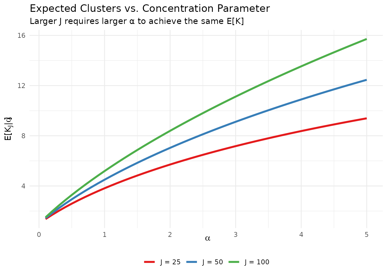

Expected number of clusters as a function of α for different sample sizes J. The approximately logarithmic relationship motivates the package’s elicitation approach.

The Low-Information Problem

When Does the Prior Matter?

In standard Bayesian analysis, priors become less influential as data accumulate—the posterior converges toward the likelihood. However, in many practical applications, the data provide limited information about $\alpha$, and the prior can substantially influence posterior inference.

Zito et al. (2024) demonstrated this sensitivity dramatically: in their Figure 1, fixing $\alpha = 1$ versus $\alpha = 5$ causes the posterior mode of $K_n$ to shift from four to eight clusters, even when data are generated from a well-separated four-component mixture. Randomizing $\alpha$ through an appropriate prior attenuates this sensitivity, but raises the question: how should that prior be specified?

Lee et al. (2025) addressed this question in the context of multisite trials by defining an informativeness index $I$: $$I = \frac{\sigma^2}{\sigma^2 + \exp\left(\frac{1}{J}\sum_{j=1}^{J} \log(\widehat{se}_j^2)\right)},$$ where $\sigma^2$ is the between-site variance and $\widehat{se}_j$ are the within-site standard errors. The index $I$ ranges from 0 to 1, with higher values indicating that the observed estimates $\hat{\tau}_j$ provide greater information about the true site effects $\tau_j$. When $I$ is small (e.g., $< 0.3$), the site-specific estimates are noisy relative to the between-site heterogeneity, and the prior on $\alpha$ can dominate the posterior.

Characteristics of Low-Information Settings

Low-information settings commonly arise in:

• Multisite trials with moderate numbers of sites ($J = 25$–$100$) and small within-site samples. Lee et al. (2025) found that for $J \leq 50$ and low $I$, even misspecified Gaussian models with appropriate posterior summaries can outperform DP models with poorly chosen priors.
• Meta-analyses with heterogeneous effect sizes and varying study precision
• Educational studies where school or classroom effects exhibit substantial variability
• Healthcare quality assessment with limited patient counts per provider

In these settings, researchers cannot simply “let the data speak”—the prior matters, and choosing it thoughtfully is essential. As Lee et al. (2025) showed, the combination of an informative prior (DP-inform) with appropriate posterior summaries outperforms diffuse approaches precisely because it incorporates meaningful prior knowledge about the expected clustering structure.

# Conceptual illustration of prior influence
# Create a schematic showing prior vs posterior at different I levels
I_levels <- c("Low (I = 0.2)", "Medium (I = 0.5)", "High (I = 0.8)")
alpha_grid <- seq(0.01, 6, length.out = 200)

# Create synthetic data for illustration
concept_data <- do.call(rbind, lapply(seq_along(I_levels), function(i) {
  I <- c(0.2, 0.5, 0.8)[i]
  prior_weight <- 1 - I
  
  # Prior: Gamma(1.5, 0.8)
  prior <- dgamma(alpha_grid, 1.5, 0.8)
  
  # "Likelihood peak" centered at alpha = 2.5
  likelihood_center <- 2.5
  likelihood_width <- 0.5 + 2 * (1 - I)  # Wider at low I
  likelihood <- dnorm(alpha_grid, likelihood_center, likelihood_width)
  
  # Posterior is mixture weighted by informativeness
  posterior <- prior_weight * prior + (1 - prior_weight) * 
               (likelihood / max(likelihood)) * max(prior)
  posterior <- posterior / (sum(posterior) * diff(alpha_grid)[1])
  
  rbind(
    data.frame(alpha = alpha_grid, density = prior, 
               Type = "Prior", Setting = I_levels[i]),
    data.frame(alpha = alpha_grid, density = posterior, 
               Type = "Posterior", Setting = I_levels[i])
  )
}))

concept_data$Setting <- factor(concept_data$Setting, levels = I_levels)
concept_data$Type <- factor(concept_data$Type, levels = c("Prior", "Posterior"))

ggplot(concept_data, aes(x = alpha, y = density, color = Type, linetype = Type)) +
  geom_line(linewidth = 1) +
  facet_wrap(~Setting, nrow = 1) +
  scale_color_manual(values = c("Prior" = "#E41A1C", "Posterior" = "#377EB8")) +
  scale_linetype_manual(values = c("Prior" = "dashed", "Posterior" = "solid")) +
  labs(x = expression(alpha),
       y = "Density",
       title = "Prior Influence Varies with Informativeness",
       subtitle = "In low-I settings, the posterior closely tracks the prior") +
  theme_minimal() +
  theme(legend.position = "bottom",
        legend.title = element_blank(),
        strip.text = element_text(face = "bold"))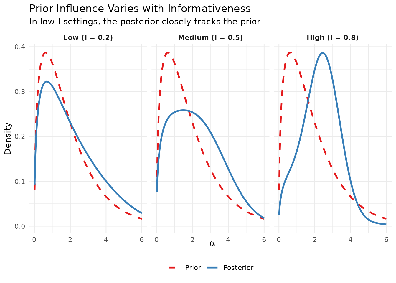

Prior influence across different informativeness levels. In low-information settings (low I), the prior’s shape substantially affects the posterior.

The K-Based Elicitation Philosophy

Speaking the Researcher’s Language

The DPprior package is built on a simple insight: while $\alpha$ is an abstract mathematical parameter, the number of clusters $K_J$ is something researchers can often reason about directly.

Consider a researcher analyzing a multisite educational trial with 50 sites. They might not have intuitions about $\alpha$, but they can likely answer questions like:

“Among your 50 sites, roughly how many distinct effect patterns or subtypes do you expect?”

“Are you fairly confident in that expectation, or quite uncertain?”

Lee et al. (2025) operationalized this approach using a chi-square distribution for $K_J$: if a researcher expects about 5 clusters, specifying $K_J \sim \chi^2(5)$ implies both a mean of 5 and a variance of 10. The package then finds Gamma parameters $(a, b)$ such that the prior on $\alpha$ induces a distribution over $K_J$ that matches these moments.

Beyond Cluster Counts: The Weight Dimension

However, Vicentini & Jermyn (2025) identified an important limitation of approaches that focus solely on $K_J$: matching a target cluster count distribution does not guarantee intuitive behavior for the cluster weights—the relative sizes of the clusters.

Consider a researcher who says “I expect about 5 clusters.” They likely imagine something like five roughly comparable groups, not a situation where one cluster contains 80% of observations while four others share the remaining 20%. Yet a prior calibrated only to match $\mathbb{E}[K_J] = 5$ might imply substantial probability of such “dominant cluster” configurations.

This insight motivates the dual-anchor framework in DPprior: researchers can additionally express beliefs about weight concentration through questions like:

“How likely is it that a single cluster would contain more than half of your sites?”

These natural questions translate directly into prior specifications:

Researcher’s Answer	Mathematical Translation
“About 5 groups”	$\mu_K = 5$ (target mean of $K_J$)
“Moderately confident”	$\text{Var}(K_J) \approx 2.5 \times \mu_K$
“Very uncertain”	$\text{Var}(K_J) \approx 5 \times \mu_K$
“Unlikely one group dominates”	$P(w_1 > 0.5) < 0.3$

From Moments to Gamma Hyperparameters

The DPprior package converts these intuitive specifications into Gamma hyperparameters $\alpha \sim \text{Gamma}(a, b)$ through a two-step process:

1. A1 (Closed-form approximation): Using the asymptotic relationship $K_J \mid \alpha \approx \text{Poisson}(\alpha \log J)$, which under a Gamma prior on $\alpha$ yields a Negative Binomial marginal for $K_J$ (Vicentini & Jermyn, 2025; Zito et al., 2024), we derive initial closed-form estimates $(a_0, b_0)$.

2. A2 (Newton refinement): Using exact moments computed via the Antoniak distribution, we refine $(a, b)$ to precisely match the target $(\mu_K, \sigma_K^2)$.

This approach—which we call DORO 2.0—extends the original DORO method (Dorazio, 2009; Lee et al., 2025) by replacing computationally expensive grid search with near-instantaneous closed-form solutions backed by Newton iteration for guaranteed accuracy. The optional dual-anchor extension further incorporates weight constraints, addressing the “unintended prior” problem identified by Vicentini & Jermyn (2025).

# Demonstrate the elicitation workflow
J <- 50
mu_K <- 5

# Method 1: Using confidence levels
fit_low <- DPprior_fit(J = J, mu_K = mu_K, confidence = "low")
#> Warning: HIGH DOMINANCE RISK: P(w1 > 0.5) = 56.3% exceeds 40%.
#>   This may indicate unintended prior behavior (RN-07).
#>   Consider using DPprior_dual() for weight-constrained elicitation.
#>   See ?DPprior_diagnostics for interpretation.
fit_med <- DPprior_fit(J = J, mu_K = mu_K, confidence = "medium")
#> Warning: HIGH DOMINANCE RISK: P(w1 > 0.5) = 49.7% exceeds 40%.
#>   This may indicate unintended prior behavior (RN-07).
#>   Consider using DPprior_dual() for weight-constrained elicitation.
#>   See ?DPprior_diagnostics for interpretation.
fit_high <- DPprior_fit(J = J, mu_K = mu_K, confidence = "high")
#> Warning: HIGH DOMINANCE RISK: P(w1 > 0.5) = 46.5% exceeds 40%.
#>   This may indicate unintended prior behavior (RN-07).
#>   Consider using DPprior_dual() for weight-constrained elicitation.
#>   See ?DPprior_diagnostics for interpretation.

# Display results
results <- data.frame(
  Confidence = c("Low", "Medium", "High"),
  VIF = c(4.0, 2.5, 1.5),
  var_K = round(c(fit_low$target$var_K, fit_med$target$var_K, 
                  fit_high$target$var_K), 2),
  a = round(c(fit_low$a, fit_med$a, fit_high$a), 3),
  b = round(c(fit_low$b, fit_med$b, fit_high$b), 3),
  E_alpha = round(c(fit_low$a/fit_low$b, fit_med$a/fit_med$b, 
                    fit_high$a/fit_high$b), 3)
)

knitr::kable(results, 
             col.names = c("Confidence", "VIF", "Var(K)", "a", "b", "E[α]"),
             caption = "Gamma hyperparameters for different confidence levels (J = 50, μ_K = 5)")

Gamma hyperparameters for different confidence levels (J = 50, μ_K = 5)

Confidence	VIF	Var(K)	a	b	E[α]
Low	4.0	20	0.518	0.341	1.519
Medium	2.5	10	1.408	1.077	1.308
High	1.5	6	3.568	2.900	1.230

What This Package Does

The DPprior package provides three core capabilities:

1. K-Based Elicitation

Convert intuitive beliefs about cluster counts into principled Gamma hyperpriors:

# The main elicitation function
fit <- DPprior_fit(
  J = 50,              # Number of observations/sites
  mu_K = 5,            # Expected number of clusters
  confidence = "medium" # Uncertainty about that expectation
)
#> Warning: HIGH DOMINANCE RISK: P(w1 > 0.5) = 49.7% exceeds 40%.
#>   This may indicate unintended prior behavior (RN-07).
#>   Consider using DPprior_dual() for weight-constrained elicitation.
#>   See ?DPprior_diagnostics for interpretation.

cat("Elicited prior: α ~ Gamma(", round(fit$a, 3), ", ", 
    round(fit$b, 3), ")\n", sep = "")
#> Elicited prior: α ~ Gamma(1.408, 1.077)

2. Dual-Anchor Control

Go beyond cluster counts to control weight concentration, addressing the “unintended prior” problem identified by Vicentini & Jermyn (2025):

# First, fit K-only prior
fit_K <- DPprior_fit(J = 50, mu_K = 5, var_K = 8)
#> Warning: HIGH DOMINANCE RISK: P(w1 > 0.5) = 48.1% exceeds 40%.
#>   This may indicate unintended prior behavior (RN-07).
#>   Consider using DPprior_dual() for weight-constrained elicitation.
#>   See ?DPprior_diagnostics for interpretation.

# Check weight behavior
p_w1 <- prob_w1_exceeds(0.5, fit_K$a, fit_K$b)
cat("K-only prior: P(w₁ > 0.5) =", round(p_w1, 3), "\n")
#> K-only prior: P(w₁ > 0.5) = 0.481

# Apply dual-anchor constraint if weight behavior is undesirable
if (p_w1 > 0.4) {
  w1_target <- list(prob = list(threshold = 0.5, value = 0.30))
  fit_dual <- DPprior_dual(fit_K, w1_target, lambda = 0.5)
  p_w1_new <- prob_w1_exceeds(0.5, fit_dual$a, fit_dual$b)
  cat("Dual-anchor prior: P(w₁ > 0.5) =", round(p_w1_new, 3), "\n")
}
#> Dual-anchor prior: P(w₁ > 0.5) = 0.438

3. Comprehensive Diagnostics

Verify that your elicited prior behaves as intended across all relevant dimensions:

# Run diagnostics
fit <- DPprior_fit(J = 50, mu_K = 5, var_K = 8, check_diagnostics = TRUE)
#> Warning: HIGH DOMINANCE RISK: P(w1 > 0.5) = 48.1% exceeds 40%.
#>   This may indicate unintended prior behavior (RN-07).
#>   Consider using DPprior_dual() for weight-constrained elicitation.
#>   See ?DPprior_diagnostics for interpretation.

# Visualize the complete prior specification
plot(fit)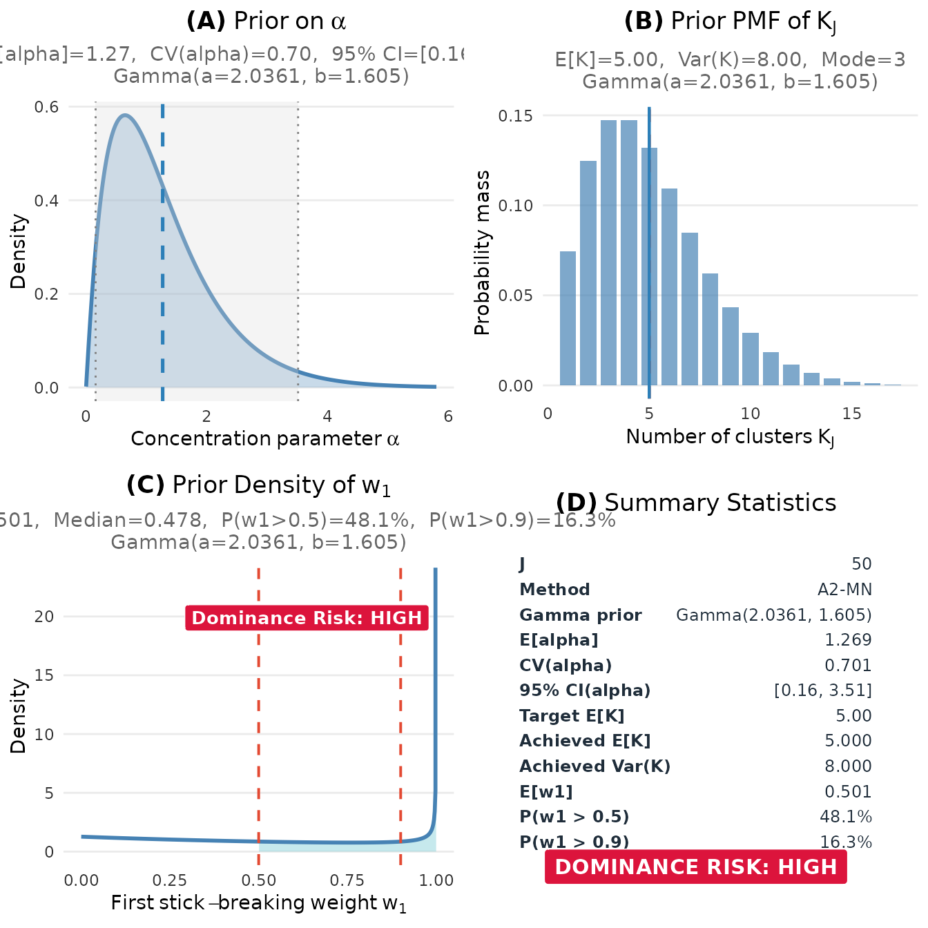

DPprior diagnostic dashboard showing the joint behavior of α, K, and w₁ under the elicited prior.

#> TableGrob (2 x 2) "dpprior_dashboard": 4 grobs
#>   z     cells              name           grob
#> 1 1 (1-1,1-1) dpprior_dashboard gtable[layout]
#> 2 2 (2-2,1-1) dpprior_dashboard gtable[layout]
#> 3 3 (1-1,2-2) dpprior_dashboard gtable[layout]
#> 4 4 (2-2,2-2) dpprior_dashboard gtable[layout]

Package Architecture

The package is organized into three layers:

Layer	Purpose	Key Functions
A. Reference Engine	Exact computation of Stirling numbers and conditional distributions	compute_log_stirling(), pmf_K_given_alpha()
B. Elicitation Engine	Mapping algorithms from moments to Gamma parameters	DPprior_a1(), DPprior_a2_newton(), DPprior_dual()
C. User Interface	User-friendly wrappers with sensible defaults	DPprior_fit(), plot(), summary()

Most users interact only with Layer C, but the underlying layers are available for advanced applications and research.

When to Use DPprior

Recommended Use Cases

The DPprior package is particularly valuable for:

• Multisite randomized trials: When analyzing heterogeneity across treatment sites with moderate $J$ (20–200 sites)

• Meta-analysis with flexible heterogeneity: When standard normal random effects may be too restrictive

• Bayesian nonparametric density estimation: When sample sizes are small enough that prior specification matters

• Mixed-effects models with flexible random effects: When exploring potential clustering among random effect distributions

When Other Approaches May Be More Appropriate

Consider alternatives when:

• Very large $J$ or streaming data: With thousands of observations, the prior on $\alpha$ becomes less influential. Sample-size-independent (SSI) approaches may be more natural.

• Highly informative data: When the likelihood provides overwhelming evidence about $\alpha$, prior specification is less critical.

• Primarily interested in prediction: DP mixture models excel at clustering and density estimation; for pure prediction tasks, other models may be more appropriate.

Road Map to the Vignettes

The DPprior package includes comprehensive documentation organized into two tracks:

Applied Researchers Track

For users who want to apply the package effectively:

Vignette	Purpose	Reading Time
Quick Start	Your first prior in 5 minutes	5 min
Applied Guide	Complete elicitation workflow	30-40 min
Dual-Anchor Framework	Control cluster counts AND weights	20-25 min
Diagnostics	Verify your prior behaves as intended	15-20 min
Case Studies	Real-world applications	30 min

Methodological Researchers Track

For users interested in the mathematical foundations:

Vignette	Purpose	Reading Time
Theory Overview	Mathematical foundations	45-60 min
Stirling Numbers	Antoniak distribution details	30 min
Approximations	A1 closed-form theory	30 min
Newton Algorithm	A2 exact moment matching	30 min
Weight Distributions	$w_1$, $\rho$, and dual-anchor	40 min
API Reference	Complete function documentation	Reference

Recommended Reading Paths

“I want to get started quickly”

→ Quick Start

“I want a systematic introduction”

→ Quick Start → Applied Guide → Dual-Anchor → Diagnostics

“I need to understand the theory”

→ Theory Overview → Stirling Numbers → Approximations → Newton Algorithm

“I need specific application examples”

→ Case Studies

Summary

The DPprior package addresses a fundamental challenge in Bayesian nonparametric modeling: how to translate domain knowledge into a principled prior on the Dirichlet Process concentration parameter $\alpha$. Key features include:

1. Intuitive elicitation: Specify priors through expected cluster counts and weight concentration, rather than abstract parameters

2. Fast computation: Closed-form approximations with Newton refinement, eliminating the need for grid search (DORO 2.0)

3. Comprehensive control: Dual-anchor framework for joint control of cluster counts and weight behavior, addressing the “unintended prior” problem identified by Vicentini & Jermyn (2025)

4. Rich diagnostics: Verification tools to ensure priors behave as intended across all relevant dimensions—not just $K_J$ but also $w_1$ and co-clustering probability $\rho$

The package is especially valuable in low-information settings—multisite trials, meta-analyses, and other applications where, as Lee et al. (2025) demonstrated, the prior on $\alpha$ can substantially influence posterior inference on site-specific effects and their distribution.

References

Antoniak, C. E. (1974). Mixtures of Dirichlet processes with applications to Bayesian nonparametric problems. The Annals of Statistics, 2(6), 1152–1174.

Dorazio, R. M. (2009). On selecting a prior for the precision parameter of Dirichlet process mixture models. Journal of Statistical Planning and Inference, 139(10), 3384–3390.

Ferguson, T. S. (1973). A Bayesian analysis of some nonparametric problems. The Annals of Statistics, 1(2), 209–230.

Lee, J., Che, J., Rabe-Hesketh, S., Feller, A., & Miratrix, L. (2025). Improving the estimation of site-specific effects and their distribution in multisite trials. Journal of Educational and Behavioral Statistics, 50(5), 731–764. https://doi.org/10.3102/10769986241254286

Sethuraman, J. (1994). A constructive definition of Dirichlet priors. Statistica Sinica, 4(2), 639–650.

Vicentini, C., & Jermyn, I. H. (2025). Prior selection for the precision parameter of Dirichlet process mixtures. arXiv:2502.00864. https://doi.org/10.48550/arXiv.2502.00864

Zito, A., Rigon, T., & Dunson, D. B. (2024). Bayesian nonparametric modeling of latent partitions via Stirling-gamma priors. arXiv:2306.02360.

---

For questions or feedback about this package, please visit the GitHub repository.