Quick Start: Your First Prior in 5 Minutes

JoonHo Lee (jlee296@ua.edu)

2026-08-22

Overview

This vignette demonstrates the fastest path to eliciting a Gamma hyperprior for the concentration parameter $\alpha$ in a Dirichlet Process mixture model. By the end of this 5-minute tutorial, you will be able to:

1. Specify your prior belief about the number of clusters
2. Convert that belief into Gamma hyperparameters
3. Visualize and verify your elicited prior

1. Minimal Example

Let’s walk through a concrete scenario. Suppose you are analyzing a multisite educational trial with 50 sites, and you expect that these sites will cluster into approximately 5 distinct effect groups. This setup mirrors the “DP-inform” prior elicitation approach used in Lee et al. (2025), who demonstrated the benefits of informative Dirichlet Process priors for estimating site-specific effects in multisite trials. While that paper relied on chi-square discrepancy measures with computationally intensive grid search, the DPprior package provides fast calibrated priors for the same elicitation task, using exact moment matching by default with a closed-form approximation available for rapid exploration.

library(DPprior)

# Just two inputs needed:
# 1. J: Number of sites (or observations for clustering)
# 2. mu_K: Expected number of clusters

fit <- DPprior_fit(J = 50, mu_K = 5, confidence = "medium")

# View the result
print(fit)
#> DPprior Prior Elicitation Result
#> ============================================= 
#> 
#> Schema: dpprior.result/1
#> Method: A2-MN (mode: a2_moment)
#> Status: converged; usable: yes; verified: yes
#> 
#> Target (J = 50):
#>   E[K_J]   = 5.0000
#>   Var(K_J) = 10.0000
#> 
#> Canonical candidate:
#>   alpha ~ Gamma(a = 1.4082, b = 1.0770)
#>   Achieved E[K_J] = 5.000000; Var(K_J) = 10.000000
#>   Maximum absolute moment residual = 5.68e-11
#> 
#> Canonical guidance: scaled component residuals and independent higher-order verification passed

That’s it! You now have a principled Gamma hyperprior for $\alpha$.

For a reusable or reviewable specification, construct the same canonical cluster-count target explicitly and pass it to the wrapper:

target_K <- DPprior_target_K(J = 50, mu_K = 5, confidence = "medium")
fit_from_target <- DPprior_fit(
  J = 50,
  target_K = target_K,
  method = "A2-MN",
  check_diagnostics = FALSE
)
fit_from_target$target$K$implied[c("mean", "variance")]
#> $mean
#> [1] 5
#> 
#> $variance
#> [1] 10

2. Understanding the Output

The DPprior_fit() function returns a canonical dpprior.result/1 object. Its scientific fields are nested; compatibility aliases are not authoritative. Let’s examine the key components:

# The Gamma hyperparameters
cat("Gamma shape (a):", round(fit$parameters$a, 4), "\n")
#> Gamma shape (a): 1.4082
cat("Gamma rate  (b):", round(fit$parameters$b, 4), "\n")
#> Gamma rate  (b): 1.077

# What these imply about alpha
alpha_mean <- fit$parameters$a / fit$parameters$b
alpha_sd <- sqrt(fit$parameters$a) / fit$parameters$b
cat("\nPrior mean of α:", round(alpha_mean, 3), "\n")
#> 
#> Prior mean of α: 1.308
cat("Prior SD of α:  ", round(alpha_sd, 3), "\n")
#> Prior SD of α:   1.102

# The target specification and decision fields
cat("\nTarget E[K]:", fit$target$K$implied$mean, "\n")
#> 
#> Target E[K]: 5
cat("Target Var(K):", round(fit$target$K$implied$variance, 2), "\n")
#> Target Var(K): 10
fit[c("status", "usable", "verified")]
#> $status
#> [1] "converged"
#> 
#> $usable
#> [1] TRUE
#> 
#> $verified
#> [1] TRUE

Interpretation: The elicited prior $\alpha \sim \text{Gamma}(a, b)$ implies that you expect around 5 clusters when sampling $J = 50$ observations, with uncertainty captured by the variance.

3. Visualizing Your Prior

The DPprior package provides built-in visualization functions to help you understand and communicate your elicited prior.

3.1 Full Dashboard View

The plot() method displays a comprehensive four-panel dashboard:

plot(fit)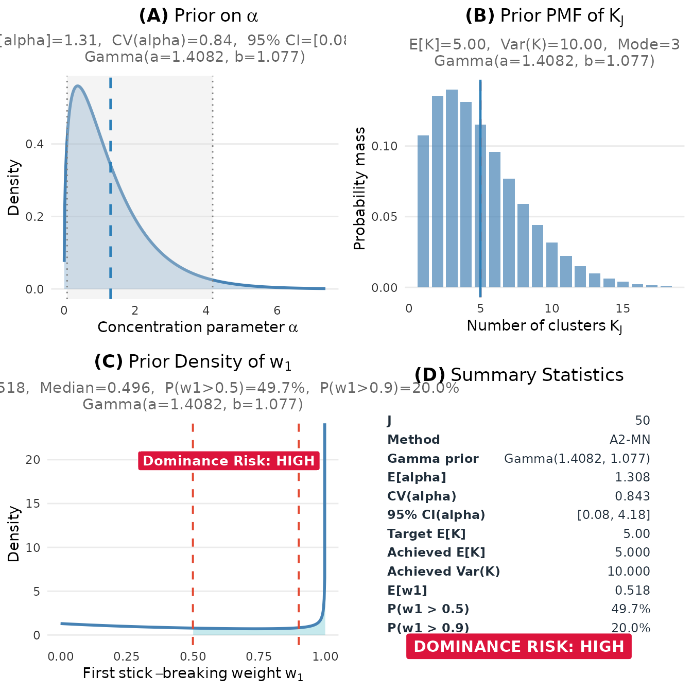

Prior elicitation dashboard showing the distributions of α, K, and w₁.

#> TableGrob (2 x 2) "dpprior_dashboard": 4 grobs
#>   z     cells              name           grob
#> 1 1 (1-1,1-1) dpprior_dashboard gtable[layout]
#> 2 2 (2-2,1-1) dpprior_dashboard gtable[layout]
#> 3 3 (1-1,2-2) dpprior_dashboard gtable[layout]
#> 4 4 (2-2,2-2) dpprior_dashboard gtable[layout]

The dashboard includes:

• Panel (A): The Gamma prior density for the concentration parameter $\alpha$, with key statistics (mean, CV, 95% CI)
• Panel (B): The implied marginal PMF of the number of clusters $K_J$, showing E[K], Var(K), and mode
• Panel (C): The prior density of the first stick-breaking weight $w_1$, with dominance risk assessment (useful for detecting overly concentrated priors)
• Panel (D): Summary statistics table consolidating all key diagnostics

3.2 Individual Plots

You can also create individual plots for more focused analysis:

plot_alpha_prior(fit)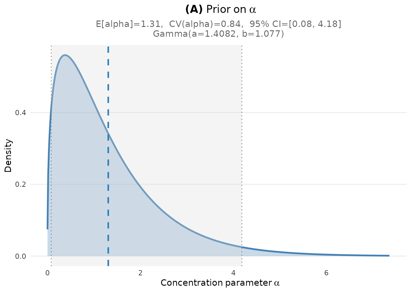

Prior density for the concentration parameter alpha.

plot_K_prior(fit)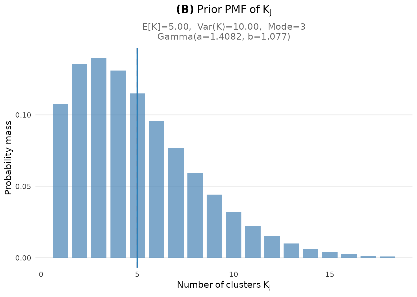

Marginal PMF of the number of clusters K.

plot_w1_prior(fit)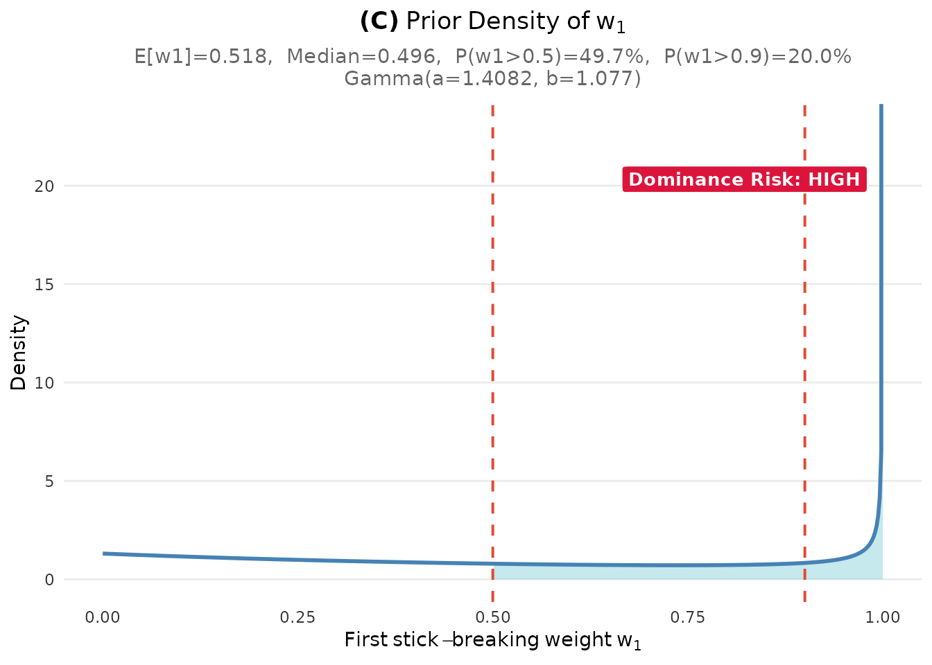

Distribution of the first stick-breaking weight w1.

4. Three Ways to Specify Your Uncertainty

The DPprior_fit() function offers flexibility in how you express your prior uncertainty about the number of clusters:

Method 1: Confidence Level (Recommended for Beginners)

The simplest approach uses qualitative confidence levels. The low-confidence case is especially diffuse, so the example requests 160 quadrature nodes and requires the package’s independent higher-order diagnostic check to pass.

# Low confidence = high uncertainty (wide prior). Use a higher quadrature
# order so this diffuse prior's diagnostics pass independent verification.
fit_low <- DPprior_fit(
  J = 50, mu_K = 5, confidence = "low", M = 160L
)

# Medium confidence = moderate uncertainty (default)
fit_med <- DPprior_fit(J = 50, mu_K = 5, confidence = "medium")

# High confidence = low uncertainty (concentrated prior)
fit_high <- DPprior_fit(J = 50, mu_K = 5, confidence = "high")

# Compare the resulting Gamma parameters
comparison <- data.frame(
  Confidence = c("Low", "Medium", "High"),
  var_K = round(c(fit_low$target$K$implied$variance,
                  fit_med$target$K$implied$variance,
                  fit_high$target$K$implied$variance), 2),
  a = round(c(fit_low$parameters$a, fit_med$parameters$a,
              fit_high$parameters$a), 3),
  b = round(c(fit_low$parameters$b, fit_med$parameters$b,
              fit_high$parameters$b), 3),
  CV_alpha = round(1/sqrt(c(fit_low$parameters$a,
                            fit_med$parameters$a,
                            fit_high$parameters$a)), 3)
)
comparison
#>   Confidence var_K     a     b CV_alpha
#> 1        Low    20 0.518 0.341    1.390
#> 2     Medium    10 1.408 1.077    0.843
#> 3       High     6 3.568 2.900    0.529

Interpretation: Higher confidence (lower uncertainty) leads to a more concentrated prior on $\alpha$, reflected in the lower coefficient of variation (CV).

Method 2: Direct Variance Specification

For users who want precise control:

# Specify variance of K directly
fit_direct <- DPprior_fit(J = 50, mu_K = 5, var_K = 10)
cat("Direct specification: var_K = 10\n")
#> Direct specification: var_K = 10
cat("  Gamma(a =", round(fit_direct$parameters$a, 3),
    ", b =", round(fit_direct$parameters$b, 3), ")\n")
#>   Gamma(a = 1.408 , b = 1.077 )

Method 3: Different Calibration Methods

For advanced users, different calibration algorithms are available:

# A2-MN (default): Exact moment matching via Newton's method
fit_newton <- DPprior_fit(J = 50, mu_K = 5, var_K = 10, method = "A2-MN")

# A1: Fast closed-form approximation (good for large J)
fit_approx <- DPprior_fit(J = 50, mu_K = 5, var_K = 10, method = "A1")

cat("A2-MN: Gamma(", round(fit_newton$parameters$a, 3), ", ",
    round(fit_newton$parameters$b, 3), ")\n", sep = "")
#> A2-MN: Gamma(1.408, 1.077)
cat("A1:    Gamma(", round(fit_approx$parameters$a, 3), ", ",
    round(fit_approx$parameters$b, 3), ")\n", sep = "")
#> A1:    Gamma(2.667, 2.608)

5. Using Your Prior in Practice

Once you have elicited your Gamma hyperparameters, you can use them in your Bayesian software of choice.

Stan

data {
  int<lower=1> J;
}
parameters {
  real<lower=0> alpha;
}
model {
  // Elicited prior from DPprior
  alpha ~ gamma(1.6, 0.816);  // Use fit$parameters$a and $b from R
}

JAGS

model {
  # Elicited prior from DPprior
  alpha ~ dgamma(1.6, 0.816)  # Note: JAGS uses rate parameterization
  
  # ... rest of your DP mixture model
}

R (for simulation)

# Draw samples from the elicited prior
n_samples <- 10000
alpha_samples <- rgamma(
  n_samples,
  shape = fit$parameters$a,
  rate = fit$parameters$b
)

cat("Summary of sampled α values:\n")
#> Summary of sampled α values:
cat("  Mean:", round(mean(alpha_samples), 3), "\n")
#>   Mean: 1.32
cat("  SD:  ", round(sd(alpha_samples), 3), "\n")
#>   SD:   1.118
cat("  95% CI: [", round(quantile(alpha_samples, 0.025), 3), ", ",
    round(quantile(alpha_samples, 0.975), 3), "]\n", sep = "")
#>   95% CI: [0.079, 4.256]

What’s Next?

This quick start covered the essentials. For more advanced topics:

• Use DPprior_dual_hard() for a verified weight inequality and DPprior_dual_soft() for an explicit fixed-scale trade-off. The retained DPprior_dual() function is a legacy equality-loss adapter, not a hard constraint certificate; it remains available throughout v2.x and will not be removed before v3.0 and a migration review.

• Applied Guide: Comprehensive elicitation workflow with sensitivity analysis

• Dual-Anchor Framework: Control both cluster count AND cluster weight concentration

• Diagnostics: Verify your prior meets your specifications

• Case Studies: Real-world examples from education, medicine, and policy research

Summary

Step	Action	Code
1	Define context	J <- 50
2	Set expected clusters	mu_K <- 5
3	Choose confidence	confidence = "medium"
4	Elicit prior	fit <- DPprior_fit(J = J, mu_K = mu_K, confidence = "medium")
5	Visualize	plot(fit)
6	Use in model	alpha ~ gamma(fit$parameters$a, fit$parameters$b)

References

Lee, J., Che, J., Rabe-Hesketh, S., Feller, A., & Miratrix, L. (2025). Improving the estimation of site-specific effects and their distribution in multisite trials. Journal of Educational and Behavioral Statistics, 50(5), 731–764. https://doi.org/10.3102/10769986241254286

---

For questions or feedback, please visit the GitHub repository.