Complete API Reference with Examples

Overview

This vignette provides a comprehensive reference for every exported function in IRTsimrel v0.3.0. Functions are organized into five categories:

Calibration Functions – The core algorithms for reliability-targeted simulation (eqc_calibrate, sac_calibrate, compare_eqc_sac).
Simulation Functions – Generators for latent abilities, item parameters, and response data (sim_latentG, sim_item_params, simulate_response_data, compare_shapes).
Reliability Functions – Low-level utilities for computing and exploring reliability (compute_rho_bar, compute_rho_tilde, compute_rho_both, compute_apc_init, check_feasibility, rho_curve, compute_reliability_tam).
S3 Methods – Print, summary, plot, coef, predict, and coercion methods for all object classes.
Deprecated Functions – Legacy aliases retained for backward compatibility (spc_calibrate, compare_eqc_spc).

For conceptual introductions, see vignette("introduction"). For applied workflow guidance, see vignette("applied-guide"). For the mathematical theory, see vignette("theory-reliability").

Citation: Lee, J.-H. (2026). Reliability-Targeted Simulation of Item Response Data: Solving the Inverse Design Problem. arXiv:2512.16012v2. https://doi.org/10.48550/arXiv.2512.16012

1. Calibration Functions

1.1 `eqc_calibrate()` – Empirical Quadrature Calibration

Implements Algorithm 1 (EQC) from Lee (2026). Given a target marginal reliability, EQC draws a large fixed quadrature sample of abilities and item parameters, maps the reliability topology over the requested log-scale interval, and applies an explicit root-selection policy. Brent’s method (uniroot()) locally polishes ordinary sign-changing crossings; boundary, tangent, plateau, and infeasible best-achievable outcomes follow their separate contracts. This is the recommended starting point for most simulation studies and targets the average-information metric.

Signature

eqc_calibrate(
  target_rho,
  n_items,
  model             = c("rasch", "2pl", "3pl"),
  latent_shape      = "normal",
  item_source       = "parametric",
  latent_params     = list(),
  item_params       = list(),
  reliability_metric = "info",
  M                 = 10000L,
  c_bounds          = c(0.3, 3),
  tol               = 1e-4,
  seed              = NULL,
  verbose           = FALSE,
  root_policy       = "lowest_increasing",
  root_controls     = list(),
  allow_tangent     = FALSE,
  allow_plateau     = FALSE
)

Parameters

Parameter	Type	Default	Description
`target_rho`	numeric	required	Target marginal reliability in (0, 1).
`n_items`	integer	required	Number of test items.
`model`	character	`"rasch"`	Measurement model: `"rasch"`, `"2pl"`, or `"3pl"` (fixed logistic convention `D = 1`).
`latent_shape`	character	`"normal"`	Shape passed to `sim_latentG()`.
`item_source`	character	`"parametric"`	Source passed to `sim_item_params()`; `"irw"` is optional external integration.
`latent_params`	list	`list()`	Additional arguments for `sim_latentG()`.
`item_params`	list	`list()`	Additional arguments for `sim_item_params()`; for 3PL, pass `guessing_params` or a custom bank with `custom_params$guessing`.
`reliability_metric`	character	`"info"`	EQC supports `"info"`/`"tilde"`; use SAC for direct `"msem"`/`"bar"` targeting.
`M`	integer	`10000L`	Quadrature sample size.
`c_bounds`	numeric(2)	`c(0.3, 3)`	Search bounds for scaling factor c.
`tol`	numeric	`1e-4`	Residual/root-polishing tolerance used by topology classification and local crossing refinement.
`seed`	integer or NULL	`NULL`	Random seed for reproducibility.
`verbose`	logical	`FALSE`	Print progress messages.
`root_policy`	character	`"lowest_increasing"`	One of `lowest_increasing`, `nearest_increasing`, `lowest_any`, or `highest_any`; the default chooses the lowest positive-slope crossing.
`root_controls`	list	`list()`	Advanced controls for the adaptive log-scale topology scan. The requested `c_bounds` are not expanded.
`allow_tangent`	logical	`FALSE`	Permit a detected tangent root to be selected by a compatible `"*_any"` policy.
`allow_plateau`	logical	`FALSE`	Permit the midpoint of a detected target plateau to be selected by a compatible `"*_any"` policy.

Return Value

An object of class "eqc_result" (a list) with elements:

Element	Description
`c_star`	Calibrated discrimination scale factor.
`target_rho`	The target reliability supplied.
`achieved_rho`	Empirical quadrature estimate at `c_star`.
`metric`	Internal metric label (`"info"`).
`model`	Model used (`"rasch"`, `"2pl"`, or `"3pl"`).
`n_items`	Number of items.
`M`	Quadrature sample size.
`theta_quad`	Length-M vector of quadrature abilities.
`theta_var`	Sample variance of `theta_quad`.
`beta_vec`	Item difficulties.
`lambda_base`	Baseline (unscaled) discriminations.
`lambda_scaled`	Discriminations scaled by `c_star`.
`guessing_vec`	Lower asymptotes (all zero for new Rasch/2PL results).
`items_base`	`item_params` object at scale = 1.
`items_calib`	`item_params` object with scaled discriminations.
`call`	The matched call.
`schema_version`, `item_scope`	Additive schema version and the fixed-form estimand scope.
`estimand_signature`, `design_signature`	Canonical estimand and realized-design provenance used in comparisons.
`misc`	Bounds, achievable range, topology, root-selection, status, and local root-polishing diagnostics.

Examples

# Rasch model with 25 items targeting rho = 0.80
eqc_res <- eqc_calibrate(
  target_rho = 0.80,
  n_items    = 25,
  model      = "rasch",
  reliability_metric = "info",
  M          = 5000L,
  seed       = 42
)
eqc_res
#> 
#> =======================================================
#>   Empirical Quadrature Calibration (EQC) Results
#> =======================================================
#> 
#> Calibration Summary:
#>   Model                        : RASCH
#>   Target reliability (rho*)    : 0.8000
#>   Achieved reliability         : 0.8000
#>   Absolute error               : 4.64e-08
#>   Scaling factor (c*)          : 0.8995
#> 
#> Design Parameters:
#>   Number of items (I)          : 25
#>   Quadrature points (M)        : 5000
#>   Reliability metric           : Average-information (tilde)
#>   Latent variance              : 1.0099
#> 
#> Convergence:
#>   Root status                  : uniroot_success
#>   Calibration status           : ok
#>   Roots detected               : 1
#>   Search bracket               : [0.300, 3.000]
#>   Bracket reliabilities        : [0.3539, 0.9550]
#> 
#> Parameter Summaries:
#>   theta:        mean = -0.014, sd = 1.005
#>   beta:         mean = 0.000, sd = 0.861, range = [-2.17, 1.45]
#>   lambda_base:  mean = 1.000, sd = 0.000
#>   lambda_scaled: mean = 0.899, sd = 0.000

# 2PL model with bimodal latent distribution
eqc_2pl <- eqc_calibrate(
  target_rho   = 0.85,
  n_items      = 30,
  model        = "2pl",
  latent_shape = "bimodal",
  reliability_metric = "info",
  M            = 5000L,
  seed         = 42
)
cat(sprintf("c* = %.4f, achieved rho = %.4f\n",
            eqc_2pl$c_star, eqc_2pl$achieved_rho))
#> c* = 1.0072, achieved rho = 0.8500

See vignette("algorithm-eqc") for a detailed walk-through.

# Fixed-form 3PL calibration: guessing is held fixed while discrimination scales
eqc_3pl <- eqc_calibrate(
  target_rho = 0.70,
  n_items = 10,
  model = "3pl",
  item_params = list(
    guessing_params = list(distribution = "fixed", value = 0.20)
  ),
  M = 2000L,
  seed = 42
)
coef(eqc_3pl)[1:4, c("beta", "lambda_base", "lambda_scaled", "guessing")]
#>         beta lambda_base lambda_scaled guessing
#> 1  0.8307240    1.215171      1.715241      0.2
#> 2  0.3022219    1.455425      2.054364      0.2
#> 3 -1.1445898    1.681011      2.372784      0.2
#> 4 -1.4265590    1.289468      1.820112      0.2

1.2 `sac_calibrate()` – Stochastic Approximation Calibration

Implements Algorithm 2 (SAC) from Lee (2026). Uses the Robbins–Monro stochastic approximation framework with Polyak–Ruppert averaging. SAC can target the MSEM-based reciprocal-information reliability and provides same-estimand validation of EQC when reliability_metric = "info".

Signature

sac_calibrate(
  target_rho,
  n_items,
  model              = c("rasch", "2pl", "3pl"),
  latent_shape       = "normal",
  item_source        = "parametric",
  latent_params      = list(),
  item_params        = list(),
  reliability_metric = c("msem", "info", "bar", "tilde"),
  c_init             = NULL,
  M_per_iter         = 500L,
  M_pre              = 10000L,
  n_iter             = 300L,
  burn_in            = NULL,
  step_params        = list(),
  c_bounds           = c(0.01, 20),
  resample_items     = TRUE,
  seed               = NULL,
  verbose            = FALSE,
  root_policy        = "lowest_increasing",
  preflight_controls = list(),
  evaluation_controls = list()
)

Parameters

Parameter	Type	Default	Description
`target_rho`	numeric	required	Target marginal reliability in (0, 1).
`n_items`	integer	required	Number of test items.
`model`	character	`"rasch"`	Measurement model: `"rasch"`, `"2pl"`, or `"3pl"` (`D = 1`).
`latent_shape`	character	`"normal"`	Shape passed to `sim_latentG()`.
`item_source`	character	`"parametric"`	Source passed to `sim_item_params()`.
`latent_params`	list	`list()`	Additional arguments for `sim_latentG()`.
`item_params`	list	`list()`	Additional arguments for `sim_item_params()`.
`reliability_metric`	character	`"msem"`	Metric: `"msem"`/`"bar"` or `"info"`/`"tilde"`.
`c_init`	numeric, `eqc_result`, or NULL	`NULL`	Initial scale. A compatible EQC object is a strict fixed-form, same-estimand warm start. With `NULL`, the selected preflight root is used for 3PL and whenever APC is unavailable.
`M_per_iter`	integer	`500L`	Monte Carlo samples per iteration.
`M_pre`	integer	`10000L`	Samples for pre-calculating latent variance.
`n_iter`	integer	`300L`	Total Robbins–Monro iterations.
`burn_in`	integer or NULL	`NULL`	Iterations to discard before averaging. Default: `floor(n_iter / 2)`.
`step_params`	list	`list()`	Step size parameters: `a` (base, default 1.0), `A` (stabilization, default 50), `gamma` (decay, default 0.67).
`c_bounds`	numeric(2)	`c(0.01, 20)`	Projection bounds for iterates.
`resample_items`	logical	`TRUE`	`FALSE` targets one fixed form; `TRUE` targets an item-superpopulation by redrawing forms.
`seed`	integer or NULL	`NULL`	Random seed.
`verbose`	logical or integer	`FALSE`	Print progress (2 for iteration-level detail).
`root_policy`	character	`"lowest_increasing"`	Root policy for the deterministic branch preflight.
`preflight_controls`	list	`list()`	Controls for topology scanning, split-form stability checks, and preflight Monte Carlo size.
`evaluation_controls`	list	`list()`	Controls for the independent post-calibration evaluation, including `M` and number of forms.

Return Value

An object of class "sac_result" (a list) with elements:

Element	Description
`c_star`	Polyak–Ruppert averaged scaling factor.
`c_final`	Final iterate value.
`target_rho`	Target reliability.
`achieved_rho`	Post-calibration reliability estimate.
`theta_var`	Pre-calculated latent variance.
`trajectory`	Numeric vector of all iterates.
`rho_trajectory`	Reliability estimates at each iteration.
`rho_update_trajectory`	Reliability sequence used in the stochastic updates.
`evaluation_trajectory`, `rho_scale_trajectory`	Scale values aligned with the reliability sequence.
`iteration_trace`	Row-wise iteration diagnostics.
`raw_trajectory`	Unprojected candidate iterates before bounds are applied.
`step_size_trajectory`	Robbins–Monro step sizes used at each iteration.
`gradient_trajectory`	Stochastic reliability residuals used for updates.
`projected`	Logical vector indicating whether each iterate hit projection bounds.
`projection_side`	Projection side for each iteration (`"lower"`, `"upper"`, or `"none"`).
`projection_count`, `projection_rate`	Projection frequency diagnostics.
`M_final`	Final post-calibration Monte Carlo sample size used for `achieved_rho`.
`metric`	Internal metric label.
`calibration_status`	Overall SAC calibration status (`"ok"` or diagnostic label).
`model`	Model used.
`n_items`	Number of items.
`n_iter`	Total iterations run.
`burn_in`	Burn-in used.
`M_per_iter`	Samples per iteration.
`M_pre`	Pre-calculation sample size.
`step_params`	Step size parameters used.
`c_bounds`	Projection bounds.
`c_init`	Initial value used.
`init_method`	Initialization method label.
`item_design`	Item draw policy used for the final calibrated design.
`item_scope`	`"fixed_form"` or `"item_superpopulation"`.
`convergence`	List of convergence diagnostics.
`beta_vec`	Item difficulties from the fixed form, or from the stored representative evaluation form for an item-superpopulation result.
`lambda_base`	Baseline discriminations.
`lambda_scaled`	Scaled discriminations.
`guessing_vec`	Item lower asymptotes (zero for new Rasch/2PL results).
`items_base`	Baseline `item_params` object.
`items_calib`	Calibrated `item_params` object.
`theta_quad`	Theta sample for post-calibration estimate.
`schema_version`, `estimand_signature`, `design_signature`	Schema and comparison provenance.
`calibration_design`, `evaluation_design`	Calibration and independent evaluation designs.
`achieved_distribution`, `achieved_se`, `representative_achieved_rho`	Holdout reliability distribution and summary.
`preflight`, `branch`	Deterministic topology scan and selected increasing-branch contract.
`requested_c_bounds`, `projection_source`	Requested interval and effective projection provenance.
`rng_provenance`, `warm_start`	RNG stream and initializer audit metadata.
`preflight_controls`, `evaluation_controls`	Normalized controls actually used.
`call`	The matched call.

Examples

# SAC with APC initialization (default)
sac_res <- sac_calibrate(
  target_rho = 0.80,
  n_items    = 25,
  model      = "rasch",
  reliability_metric = "msem",
  n_iter     = 200L,
  M_per_iter = 500L,
  M_pre      = 5000L,
  seed       = 42,
  verbose    = FALSE
)
cat(sprintf("SAC c* = %.4f, achieved rho = %.4f\n",
            sac_res$c_star, sac_res$achieved_rho))
#> SAC c* = 1.0504, achieved rho = 0.8250

# Warm start from EQC result (recommended workflow)
sac_warm <- sac_calibrate(
  target_rho = 0.80,
  n_items    = 25,
  model      = "rasch",
  reliability_metric = "info",
  c_init     = eqc_res,
  resample_items = FALSE,
  n_iter     = 100L,
  M_per_iter = 500L,
  M_pre      = 5000L,
  seed       = 42,
  verbose    = FALSE
)
cat(sprintf("EQC c* = %.4f, SAC c* = %.4f\n",
            eqc_res$c_star, sac_warm$c_star))
#> EQC c* = 0.8995, SAC c* = 0.8998

See vignette("algorithm-sac") for convergence tuning details.

1.3 `compare_eqc_sac()` – Compare Calibration Results

Computes agreement diagnostics between EQC and SAC calibration results. For same-estimand validation of an EQC result, the SAC result should use reliability_metric = "info" and comparable design inputs.

Signature

compare_eqc_sac(eqc_result, sac_result, verbose = TRUE)

Parameters

Parameter	Type	Default	Description
`eqc_result`	`eqc_result`	required	Output from `eqc_calibrate()`.
`sac_result`	`sac_result` or legacy `spc_result`	required	Output from `sac_calibrate()` or deprecated `spc_calibrate()`.
`verbose`	logical	`TRUE`	Print comparison summary.

The comparison warns when metric, model, test length, or calibration status metadata differ. Use reliability_metric = "info" in SAC for same-estimand validation of EQC.

Return Value

A list (returned invisibly) with components:

Element	Description
`c_eqc`	Calibrated `c*` from EQC.
`c_sac`	Calibrated `c*` from SAC.
`diff_abs`	Absolute difference between the two `c*` values.
`diff_pct`	Percent difference relative to EQC.
`agreement`	`TRUE` or `FALSE` when agreement is validly evaluated; `NA` when comparability or calibration status requires withholding it.
`target_rho`	Shared target reliability.
`achieved_eqc`	Achieved reliability from EQC.
`achieved_sac`	Achieved reliability from SAC.
`achieved_diff_abs`	Absolute difference between achieved reliability estimates.
`metric_eqc`, `metric_sac`	Metric labels used by each result.
`model_eqc`, `model_sac`	Model labels used by each result.
`n_items_eqc`, `n_items_sac`	Test lengths used by each result.
`eqc_status`, `sac_status`, `sac_status_flags`	Calibration status metadata.
`comparable`	Whether the stored estimand and design contracts match.
`comparability_reasons`	Stable reason codes when contracts are not comparable.
`agreement_status`, `agreement_reasons`	Whether agreement was evaluated and why it was withheld otherwise.
`eqc_contract`, `sac_contract`	Normalized contracts used for the comparison decision.

Examples

# Compare results from the two algorithms
comp <- compare_eqc_sac(eqc_res, sac_warm, verbose = TRUE)
#> 
#> =======================================================
#>   EQC vs SAC Comparison
#> =======================================================
#> 
#>   Target reliability  : 0.8000
#>   EQC c*              : 0.899499
#>   SAC c*              : 0.899822
#>   Absolute difference : 0.000323
#>   Percent difference  : 0.04%
#>   EQC achieved rho    : 0.8000
#>   SAC achieved rho    : 0.8002
#>   Comparable           : YES
#>   Agreement (< 5%)    : YES
#>   Agreement status     : evaluated
#>   EQC status          : uniroot_success
#>   SAC status          : ok
#>   SAC status flags    : ok
#> 
cat(sprintf("Agreement: %s (%.2f%% difference)\n",
            ifelse(comp$agreement, "YES", "NO"), comp$diff_pct))
#> Agreement: YES (0.04% difference)

2. Simulation Functions

2.1 `sim_latentG()` – Simulate Latent Ability Distributions

Generates latent abilities from a flexible family of pre-standardized distributions. Each built-in shape is mathematically constructed to have mean 0 and variance 1, so changes in distributional shape do not alter the scale.

Signature

sim_latentG(
  n,
  shape              = c("normal", "bimodal", "trimodal", "multimodal",
                          "skew_pos", "skew_neg", "heavy_tail",
                          "light_tail", "uniform", "floor", "ceiling",
                          "custom"),
  sigma              = 1,
  mu                 = 0,
  xcov               = NULL,
  beta               = NULL,
  shape_params       = list(),
  mixture_spec       = NULL,
  standardize_custom = TRUE,
  seed               = NULL,
  return_z           = TRUE
)

Parameters

Parameter	Type	Default	Description
`n`	integer	required	Number of persons.
`shape`	character	`"normal"`	Distributional shape (see table below).
`sigma`	numeric	`1`	Standard deviation of the residual latent trait.
`mu`	numeric	`0`	Grand mean of latent abilities.
`xcov`	matrix, data.frame, or NULL	`NULL`	Optional covariate data (`n` rows).
`beta`	numeric or NULL	`NULL`	Regression coefficients for `xcov`.
`shape_params`	list	`list()`	Shape-specific parameters (see below).
`mixture_spec`	list or NULL	`NULL`	For `shape = "custom"`: `weights`, `means`, `sds`.
`standardize_custom`	logical	`TRUE`	Standardize custom mixtures to mean 0, variance 1.
`seed`	integer or NULL	`NULL`	Random seed.
`return_z`	logical	`TRUE`	Include standardized draws in output.

Available shapes:

Shape	Description	Key Parameters
`"normal"`	Standard normal	–
`"bimodal"`	Symmetric two-component mixture	`delta` (mode separation, default 0.8)
`"trimodal"`	Symmetric three-component mixture	`w0` (central weight, default 1/3), `m` (side means, default 1.2)
`"multimodal"`	Symmetric four-component mixture	`m1`, `m2`, `w_inner`
`"skew_pos"`	Right-skewed (standardized Gamma)	`k` (shape, default 4)
`"skew_neg"`	Left-skewed (negated Gamma)	`k` (shape, default 4)
`"heavy_tail"`	Heavy-tailed (standardized Student-t)	`df` (degrees of freedom, default 5)
`"light_tail"`	Light-tailed (platykurtic mixture)	–
`"uniform"`	Uniform on [-sqrt(3), sqrt(3)]	–
`"floor"`	Floor effect	`w_floor` (default 0.3), `m_floor` (default -1.5)
`"ceiling"`	Ceiling effect	`w_ceil` (default 0.3), `m_ceil` (default 1.5)
`"custom"`	User-specified mixture	See `mixture_spec`

Return Value

An object of class "latent_G" (a list) with elements:

Element	Description
`theta`	Numeric vector of simulated latent abilities.
`z`	Standardized draws (if `return_z = TRUE`).
`eta_cov`	Covariate linear predictor (0 if no covariates).
`mu`	Grand mean.
`sigma`	Scale parameter.
`shape`	Shape label.
`shape_params`	Shape parameters used.
`mixture_spec`	Custom mixture definition, present when `shape = "custom"`.
`n`	Sample size.
`sample_moments`	List: `mean`, `sd`, `skewness`, `kurtosis`.

Examples

# Standard normal abilities
g_norm <- sim_latentG(n = 2000, shape = "normal", seed = 42)
cat(sprintf("Mean = %.3f, SD = %.3f, Skew = %.3f, Kurt = %.3f\n",
            g_norm$sample_moments$mean,
            g_norm$sample_moments$sd,
            g_norm$sample_moments$skewness,
            g_norm$sample_moments$kurtosis))
#> Mean = -0.016, SD = 0.994, Skew = 0.013, Kurt = 0.056

# Bimodal distribution with strong separation
g_bimod <- sim_latentG(
  n            = 2000,
  shape        = "bimodal",
  shape_params = list(delta = 0.9),
  seed         = 42
)
cat(sprintf("Bimodal: Mean = %.3f, SD = %.3f, Kurt = %.3f\n",
            g_bimod$sample_moments$mean,
            g_bimod$sample_moments$sd,
            g_bimod$sample_moments$kurtosis))
#> Bimodal: Mean = -0.017, SD = 0.989, Kurt = -1.298

# Positively skewed distribution
g_skew <- sim_latentG(
  n            = 2000,
  shape        = "skew_pos",
  shape_params = list(k = 3),
  seed         = 42
)
cat(sprintf("Skew_pos: Skewness = %.3f\n",
            g_skew$sample_moments$skewness))
#> Skew_pos: Skewness = 1.152

# Custom three-component mixture
g_custom <- sim_latentG(
  n            = 2000,
  shape        = "custom",
  mixture_spec = list(
    weights = c(0.3, 0.5, 0.2),
    means   = c(-1.5, 0, 2),
    sds     = c(0.5, 0.7, 0.5)
  ),
  seed = 42
)
cat(sprintf("Custom: Mean = %.3f, SD = %.3f\n",
            g_custom$sample_moments$mean,
            g_custom$sample_moments$sd))
#> Custom: Mean = 0.011, SD = 0.996

See vignette("latent-distributions") for detailed shape comparisons.

2.2 `sim_item_params()` – Simulate Item Parameters

Generates item difficulty and discrimination parameters for IRT models. Supports multiple sources (parametric default, optional IRW, hierarchical, custom) and methods for inducing difficulty–discrimination correlation.

Signature

sim_item_params(
  n_items,
  model                 = c("rasch", "2pl", "3pl"),
  source                = c("parametric", "irw", "hierarchical", "custom"),
  method                = c("copula", "conditional", "independent"),
  n_forms               = 1L,
  difficulty_params     = list(),
  discrimination_params = list(),
  hierarchical_params   = list(),
  custom_params         = list(),
  scale                 = 1,
  center_difficulties   = TRUE,
  seed                  = NULL,
  guessing_params       = list()
)

Parameters

Parameter	Type	Default	Description
`n_items`	integer	required	Number of items per form.
`model`	character	`"rasch"`	`"rasch"`, `"2pl"`, or `"3pl"`.
`source`	character	`"parametric"`	`"parametric"`, optional `"irw"`, `"hierarchical"`, or `"custom"`.
`method`	character	`"copula"`	For 2PL/3PL discrimination generation: `"copula"`, `"conditional"`, or `"independent"`.
`n_forms`	integer	`1L`	Number of parallel test forms.
`difficulty_params`	list	`list()`	For parametric: `mu` (default 0), `sigma` (default 1), `distribution` (default `"normal"`).
`discrimination_params`	list	`list()`	For 2PL/3PL: `mu_log` (default 0), `sigma_log` (default 0.3), `rho` (default -0.3).
`hierarchical_params`	list	`list()`	For hierarchical: `mu` (2-vector), `tau` (2-vector), `rho`.
`custom_params`	list	`list()`	For custom: `beta`, `lambda`, and, for 3PL, `guessing` (vectors or functions).
`scale`	numeric	`1`	Global discrimination scaling factor.
`center_difficulties`	logical	`TRUE`	Center difficulties to sum to zero.
`seed`	integer or NULL	`NULL`	Random seed.
`guessing_params`	list	`list()`	3PL lower-asymptote generator; supported distributions are `"fixed"`, `"uniform"`, and `"beta"`, with bounds constrained below 1. Must remain empty for Rasch/2PL; nonempty guessing input is rejected.

Return Value

An object of class "item_params" (a list) with elements:

Element	Description
`data`	Data frame: `form_id`, `item_id`, `beta`, `lambda`, `lambda_unscaled`, and `guessing` for 3PL.
`model`	Model type.
`source`	Source used.
`method`	Method for discriminations (NA for Rasch or hierarchical).
`n_items`	Items per form.
`n_forms`	Forms generated.
`scale`	Scale factor applied.
`centered`	Whether difficulties were centered.
`params`	Normalized parameters used for generation, including the 3PL guessing specification when applicable.
`achieved`	Achieved statistics (correlations, moments).

Examples

# Rasch items with parametric difficulties
items_rasch <- sim_item_params(
  n_items = 25,
  model   = "rasch",
  source  = "parametric",
  seed    = 42
)
items_rasch
#> Item Parameters Object
#> ======================
#>   Model          : RASCH
#>   Source         : parametric
#>   Items per form : 25
#>   Number of forms: 1
#>   Scale factor   : 1.0000
#>   Centered       : Yes
#> 
#> Difficulty (beta):
#>   Mean: 0.0000, SD: 1.3064, Range: [-2.8440, 2.0991]

# 2PL items with copula-induced correlation
items_2pl <- sim_item_params(
  n_items               = 30,
  model                 = "2pl",
  source                = "parametric",
  method                = "copula",
  discrimination_params = list(rho = -0.3, mu_log = 0, sigma_log = 0.3),
  seed                  = 42
)
cat(sprintf("Achieved Spearman r(beta, log-lambda) = %.3f\n",
            items_2pl$achieved$overall$cor_spearman_pooled))
#> Achieved Spearman r(beta, log-lambda) = -0.378

# Hierarchical 2PL (Glas & van der Linden style)
items_hier <- sim_item_params(
  n_items              = 25,
  model                = "2pl",
  source               = "hierarchical",
  hierarchical_params  = list(mu = c(0, 0), tau = c(0.25, 1), rho = -0.3),
  seed                 = 42
)
head(as.data.frame(items_hier))
#>   form_id item_id       beta    lambda lambda_unscaled
#> 1       1       1  1.1864454 0.9930935       0.9930935
#> 2       1       2 -0.7521311 1.1116693       1.1116693
#> 3       1       3  0.2039055 1.4755926       1.4755926
#> 4       1       4  0.4317000 0.8526922       0.8526922
#> 5       1       5  0.2238748 1.1270078       1.1270078
#> 6       1       6 -0.3070683 0.9052717       0.9052717

# Custom user-supplied parameters
items_custom <- sim_item_params(
  n_items       = 10,
  model         = "2pl",
  source        = "custom",
  custom_params = list(
    beta   = seq(-2, 2, length.out = 10),
    lambda = rep(1.2, 10)
  ),
  seed = 42
)
head(as.data.frame(items_custom))
#>   form_id item_id       beta lambda lambda_unscaled
#> 1       1       1 -2.0000000    1.2             1.2
#> 2       1       2 -1.5555556    1.2             1.2
#> 3       1       3 -1.1111111    1.2             1.2
#> 4       1       4 -0.6666667    1.2             1.2
#> 5       1       5 -0.2222222    1.2             1.2
#> 6       1       6  0.2222222    1.2             1.2

See vignette("item-parameters") for a complete discussion of sources and methods.

items_3pl <- sim_item_params(
  n_items = 12,
  model = "3pl",
  guessing_params = list(distribution = "uniform", min = 0.15, max = 0.25),
  seed = 42
)
head(as.data.frame(items_3pl)[, c("beta", "lambda", "guessing")])
#>         beta    lambda  guessing
#> 1  0.6155849 0.4734144 0.2175607
#> 2 -1.3200717 1.7051314 0.2482817
#> 3 -0.3922451 0.9426343 0.2259544
#> 4 -0.1225110 0.5949993 0.2066488
#> 5 -0.3511052 0.9609983 0.2349690
#> 6 -0.8614981 1.5701155 0.1689474

2.3 `simulate_response_data()` – Generate Response Matrices

Simulates binary (0/1) item response data using calibrated parameters from eqc_calibrate() or sac_calibrate(). This is the final step before external validation (e.g., with TAM).

The function always uses the normalized item design stored in the calibration result. For a fixed-form result this is that calibrated form. For an SAC item_scope = "item_superpopulation" result, it is one stored representative evaluation form: this call does not redraw a new form and does not itself simulate the aggregate item-superpopulation estimand.

Signature

simulate_response_data(
  result,
  n_persons,
  latent_shape  = "normal",
  latent_params = list(),
  seed          = NULL
)

Parameters

Parameter	Type	Default	Description
`result`	`eqc_result`, `sac_result`, or legacy `spc_result`	required	Calibration result object.
`n_persons`	integer	required	Number of simulated examinees.
`latent_shape`	character	`"normal"`	Shape for `sim_latentG()`.
`latent_params`	list	`list()`	Additional arguments for `sim_latentG()`.
`seed`	integer or NULL	`NULL`	Random seed.

Return Value

A list with components:

Element	Description
`response_matrix`	N x I matrix of binary responses (column names: `item1`, …, `itemI`).
`theta`	True latent abilities (length N).
`beta`	Item difficulties (length I).
`lambda`	Scaled item discriminations (length I).
`guessing`	Item lower asymptotes (length I; zeros for Rasch/2PL).
`provenance`	Calibration and simulation metadata for reproducible audit trails.

The provenance field includes result_class, c_star, target_rho, achieved_rho, metric, model, n_items, calibration_status, status_flags, item_design, item_source, calibration_call, simulation_seed, n_persons, latent_shape, and latent_params. calibration_status is a scalar status label; status_flags is always a character vector so EQC, SAC, and legacy SPC provenance can be handled uniformly. The provenance also records schema_version, item_scope, design_signature, and item-parameter provenance.

Examples

# Generate 500 examinees from EQC calibration
sim_data <- simulate_response_data(
  result    = eqc_res,
  n_persons = 500,
  seed      = 123
)
cat(sprintf("Response matrix: %d persons x %d items\n",
            nrow(sim_data$response_matrix),
            ncol(sim_data$response_matrix)))
#> Response matrix: 500 persons x 25 items
cat(sprintf("Mean proportion correct: %.3f\n",
            mean(sim_data$response_matrix)))
#> Mean proportion correct: 0.502
sim_data$provenance[c("metric", "calibration_status", "status_flags",
                      "item_source", "simulation_seed", "latent_shape")]
#> $metric
#> [1] "info"
#> 
#> $calibration_status
#> [1] "uniroot_success"
#> 
#> $status_flags
#> [1] "uniroot_success"
#> 
#> $item_source
#> [1] "parametric"
#> 
#> $simulation_seed
#> [1] 123
#> 
#> $latent_shape
#> [1] "normal"

# Generate from SAC result with skewed abilities
sim_data2 <- simulate_response_data(
  result       = sac_warm,
  n_persons    = 500,
  latent_shape = "skew_pos",
  seed         = 123
)
cat(sprintf("Theta skewness: %.3f\n",
            mean(((sim_data2$theta - mean(sim_data2$theta)) /
                    sd(sim_data2$theta))^3)))
#> Theta skewness: 0.906

2.4 `compare_shapes()` – Compare Distribution Shapes

Generates and compares multiple latent distributions side-by-side using faceted density plots. Requires the ggplot2 package.

Signature

compare_shapes(
  n      = 2000,
  shapes = c("normal", "bimodal", "trimodal",
             "skew_pos", "skew_neg", "heavy_tail",
             "uniform"),
  sigma  = 1,
  seed   = NULL
)

Parameters

Parameter	Type	Default	Description
`n`	integer	`2000`	Sample size per distribution.
`shapes`	character vector	(see above)	Shapes to compare.
`sigma`	numeric	`1`	Common scale parameter.
`seed`	integer or NULL	`NULL`	Random seed.

Return Value

A ggplot object with faceted density plots, one panel per shape. A dashed red line shows the N(0,\sigma^2) reference density.

Example

p <- compare_shapes(
  n      = 2000,
  shapes = c("normal", "bimodal", "skew_pos", "heavy_tail"),
  seed   = 42
)
print(p)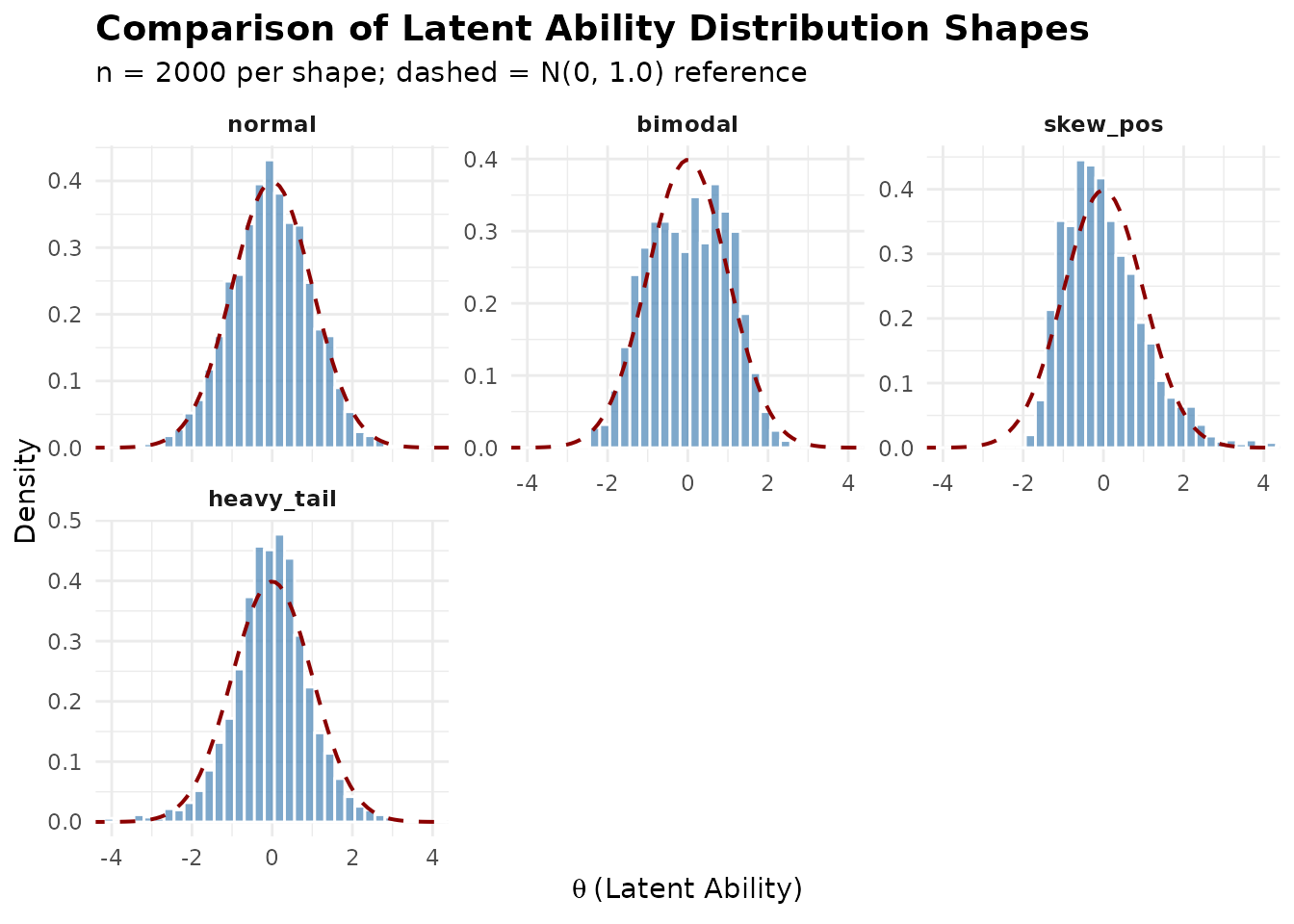

Faceted density plots comparing normal, bimodal, skewed, and heavy-tailed latent distributions.

Comparison of latent distribution shapes.

See vignette("latent-distributions") for extended shape comparisons.

3. Reliability Functions

Notation crosswalk. The package field rho_tilde corresponds to the average-information reliability \tilde{\rho} and is selected with reliability_metric = "info" or "tilde". The package field rho_bar corresponds to the manuscript’s MSEM-based reliability \bar{w} and is selected with reliability_metric = "msem" or "bar". The name rho_bar is an API label for \bar{w}, not a separate \bar{\rho} estimand.

3.1 `compute_rho_bar()` – MSEM-Based Marginal Reliability

Computes the MSEM-based marginal reliability using the reciprocal-information MSEM convention described in vignette("theory-reliability").

Signature

compute_rho_bar(
  c, theta_vec, beta_vec, lambda_base, theta_var = NULL,
  guessing = NULL, weights = NULL, return_diagnostics = FALSE
)

Parameters

Parameter	Type	Default	Description
`c`	numeric	required	Global discrimination scaling factor.
`theta_vec`	numeric vector	required	Abilities.
`beta_vec`	numeric vector	required	Item difficulties.
`lambda_base`	numeric vector	required	Baseline discriminations (before scaling).
`theta_var`	numeric or NULL	`NULL`	Pre-calculated theta variance. If `NULL`, computed from `theta_vec`.
`guessing`	numeric vector or NULL	`NULL`	Item lower asymptotes; `NULL` is the exact zero-guessing path.
`weights`	numeric vector or NULL	`NULL`	Optional non-negative integration weights, normalized internally.
`return_diagnostics`	logical	`FALSE`	Return the estimate together with numerical diagnostics instead of a scalar.

Return Value

A numeric scalar by default. With return_diagnostics = TRUE, a list contains the reliability estimate together with variance, integration, and numerical stability diagnostics.

Example

set.seed(1)
theta <- rnorm(2000)
beta  <- rnorm(20)
lambda0 <- rep(1, 20)

rho_bar_val <- compute_rho_bar(c = 1.0, theta, beta, lambda0)
cat(sprintf("rho_bar at c=1: %.4f\n", rho_bar_val))
#> rho_bar at c=1: 0.7856

3.2 `compute_rho_tilde()` – Average-Information Reliability

Computes the average-information reliability using the arithmetic mean of test information. This is the recommended metric for EQC.

Signature

compute_rho_tilde(
  c, theta_vec, beta_vec, lambda_base, theta_var = NULL,
  guessing = NULL, weights = NULL, return_diagnostics = FALSE
)

Parameters and return value are identical to compute_rho_bar() above; only the internal formula differs.

Example

rho_tilde_val <- compute_rho_tilde(c = 1.0, theta, beta, lambda0)
cat(sprintf("rho_tilde at c=1: %.4f\n", rho_tilde_val))
#> rho_tilde at c=1: 0.7931

# Jensen's inequality: rho_tilde >= rho_bar
cat(sprintf("rho_tilde >= rho_bar: %s\n",
            ifelse(rho_tilde_val >= rho_bar_val, "TRUE", "FALSE")))
#> rho_tilde >= rho_bar: TRUE

3.3 `compute_rho_both()` – Both Metrics in a Single Pass

Computes both reliability metrics from a single set of matrix computations, avoiding redundant M x I operations.

Signature

compute_rho_both(
  c, theta_vec, beta_vec, lambda_base, theta_var = NULL,
  guessing = NULL, weights = NULL, return_diagnostics = FALSE
)

Parameters are identical to compute_rho_bar(). The return value is a named list.

Return Value

Element	Description
`rho_tilde`	Average-information reliability.
`rho_bar`	MSEM-based reliability.

Example

both <- compute_rho_both(c = 1.0, theta, beta, lambda0)
cat(sprintf("rho_tilde = %.4f, rho_bar = %.4f, gap = %.4f\n",
            both$rho_tilde, both$rho_bar,
            both$rho_tilde - both$rho_bar))
#> rho_tilde = 0.7931, rho_bar = 0.7856, gap = 0.0075

3.4 `compute_apc_init()` – Analytic Pre-Calibration

Computes an initial scaling factor using a closed-form approximation under Gaussian Rasch assumptions. Used internally by sac_calibrate() when c_init = NULL.

Signature

compute_apc_init(target_rho, n_items, sigma_beta = 1.0)

Parameters

Parameter	Type	Default	Description
`target_rho`	numeric	required	Target reliability.
`n_items`	integer	required	Number of items.
`sigma_beta`	numeric	`1.0`	SD of item difficulties.

Return Value

A numeric scalar: the initial scaling factor (bounded to [0.1, 10]).

Example

# Compare APC estimates across test lengths
for (I in c(10, 20, 30, 50)) {
  c0 <- compute_apc_init(target_rho = 0.80, n_items = I)
  cat(sprintf("  I = %2d: c_init = %.4f\n", I, c0))
}
#>   I = 10: c_init = 2.0988
#>   I = 20: c_init = 1.4841
#>   I = 30: c_init = 1.2117
#>   I = 50: c_init = 0.9386

3.5 `check_feasibility()` – Feasibility Screening

Screens whether a target reliability is attainable in one generated finite Monte Carlo design by computing the empirical reliability range across a set of scaling factors. Run this before calibration to avoid wasting time on infeasible targets.

The classification is conditional on that finite theta sample. For latent_shape = "heavy_tail", a numeric MSEM range is only a finite-grid sensitivity result: the corresponding population MSEM functional can be non-integrable, so this function does not certify population feasibility.

Signature

check_feasibility(
  n_items,
  model         = c("rasch", "2pl", "3pl"),
  latent_shape  = "normal",
  item_source   = "parametric",
  c_bounds      = c(0.1, 10),
  M             = 10000L,
  seed          = NULL,
  latent_params = list(),
  item_params   = list(),
  target_rho    = NULL,
  verbose       = TRUE
)

Parameters

Parameter	Type	Default	Description
`n_items`	integer	required	Number of items.
`model`	character	`"rasch"`	`"rasch"`, `"2pl"`, or `"3pl"`.
`latent_shape`	character	`"normal"`	Latent distribution shape.
`item_source`	character	`"parametric"`	Item parameter source.
`c_bounds`	numeric(2)	`c(0.1, 10)`	Scaling factor range to evaluate.
`M`	integer	`10000L`	Monte Carlo sample size.
`seed`	integer or NULL	`NULL`	Random seed.
`latent_params`	list	`list()`	Additional arguments for `sim_latentG()`.
`item_params`	list	`list()`	Additional arguments for `sim_item_params()`.
`target_rho`	numeric or NULL	`NULL`	Optional target reliability to classify as feasible or infeasible.
`verbose`	logical	`TRUE`	Print results.

Return Value

An object of class "feasibility_check" (returned invisibly) with:

Element	Description
`rho_range_info`	Empirical range computed by the configured finite scan; provisional if topology is unresolved.
`rho_range_msem`	Empirical range computed by the configured finite scan; provisional if unresolved and finite-grid only for `heavy_tail`.
`rho_bounds_info`	Boundary reliabilities for the information metric.
`rho_bounds_msem`	Boundary reliabilities for the MSEM metric.
`rho_info_max_c`	Scale at the maximum information reliability detected by the configured scan; provisional if topology is unresolved.
`rho_msem_max_c`	Scale at the maximum MSEM reliability detected by the configured scan; provisional if topology is unresolved.
`target_rho`	Optional target reliability supplied.
`target_status_info`	Feasibility classification for `target_rho` under the information metric.
`target_status_msem`	Feasibility classification for `target_rho` under the MSEM metric.
`topology_info`, `topology_msem`	Configured log-grid scans, roots, extrema, branches, evaluation counts, and resolution status.
`target_status_info_canonical`, `target_status_msem_canonical`	Canonical status: feasible, below/above range, or uncertain.
`root_count_info`, `root_count_msem`	Number of detected roots for each metric.
`admissible_root_count_info`, `admissible_root_count_msem`	Number of detected roots on admissible increasing branches.
`best_achievable_info`, `best_achievable_msem`	Closest detected scale/reliability point and target gap.
`n_items`	Number of items.
`model`	Model.
`latent_shape`	Latent shape.
`c_bounds`	Evaluated range.
`M`	Sample size.
`theta_var`	Estimated latent variance.

Example

feas <- check_feasibility(
  n_items    = 25,
  model      = "rasch",
  M          = 5000L,
  target_rho = 0.85,
  seed       = 42,
  verbose    = FALSE
)
cat(sprintf("rho_tilde range: [%.4f, %.4f]\n",
            feas$rho_range_info[1], feas$rho_range_info[2]))
#> rho_tilde range: [0.0591, 0.9872]
cat(sprintf("rho_bar range:   [%.4f, %.4f]\n",
            feas$rho_range_msem[1], feas$rho_range_msem[2]))
#> rho_bar range:   [0.0002, 0.9146]

cat(sprintf("rho=0.85 status (info): %s\n",
            feas$target_status_info))
#> rho=0.85 status (info): feasible
cat(sprintf("rho=0.85 status (msem): %s\n",
            feas$target_status_msem))
#> rho=0.85 status (msem): feasible

3.6 `rho_curve()` – Reliability as a Function of Scaling Factor

Computes and optionally plots a finite-sample reliability curve across a grid of scaling factor values. It helps visualize the relationship between discrimination strength and measurement precision for that generated design. With latent_shape = "heavy_tail", an MSEM curve is finite-grid sensitivity evidence only and does not establish that the population MSEM functional is finite.

Signature

rho_curve(
  c_values      = seq(0.1, 5, length.out = 50),
  n_items,
  model         = c("rasch", "2pl", "3pl"),
  latent_shape  = "normal",
  item_source   = "parametric",
  metric        = c("both", "info", "msem"),
  M             = 5000L,
  seed          = NULL,
  latent_params = list(),
  item_params   = list(),
  plot          = TRUE
)

Parameters

Parameter	Type	Default	Description
`c_values`	numeric vector	`seq(0.1, 5, length.out = 50)`	Grid of scaling factor values.
`n_items`	integer	required	Number of items.
`model`	character	`"rasch"`	`"rasch"`, `"2pl"`, or `"3pl"`.
`latent_shape`	character	`"normal"`	Latent distribution shape.
`item_source`	character	`"parametric"`	Item parameter source.
`metric`	character	`"both"`	Which metric(s): `"both"`, `"info"`, or `"msem"`.
`M`	integer	`5000L`	Monte Carlo sample size.
`seed`	integer or NULL	`NULL`	Random seed.
`latent_params`	list	`list()`	Additional arguments for `sim_latentG()`.
`item_params`	list	`list()`	Additional arguments for `sim_item_params()`.
`plot`	logical	`TRUE`	Create a plot.

Return Value

A data frame of class "rho_curve", always returned invisibly, with columns c, rho_tilde, and/or rho_bar depending on the metric argument. When plot = TRUE, the plot is drawn as a side effect.

Example

curve_data <- rho_curve(
  c_values = seq(0.2, 4, length.out = 40),
  n_items  = 25,
  model    = "rasch",
  metric   = "both",
  M        = 5000L,
  seed     = 42,
  plot     = TRUE
)

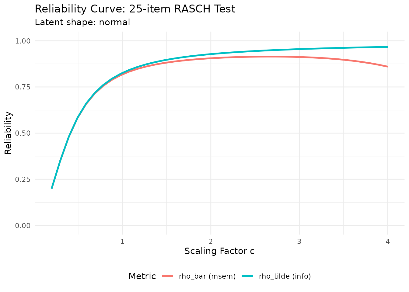
Reliability curve showing average-information and MSEM metrics over scaling factors for a 25-item Rasch test.

Reliability curve for a 25-item Rasch test.

# Inspect the data
head(curve_data)
#> Reliability Curve
#> =================
#>   Items: 25 | Model: RASCH | Metric: both
#>   c range: [0.20, 0.69] (6 points)
#>   rho_tilde range: [0.1989, 0.7174]
#>   rho_bar range  : [0.1989, 0.7139]
#> 
#>           c rho_tilde   rho_bar
#> 1 0.2000000 0.1988965 0.1988657
#> 2 0.2974359 0.3500759 0.3498742
#> 3 0.3948718 0.4807284 0.4800963
#> 4 0.4923077 0.5827614 0.5814095
#> 5 0.5897436 0.6596796 0.6573608
#> 6 0.6871795 0.7174113 0.7139425

3.7 `compute_reliability_tam()` – TAM-Based Validation

Fits a Rasch or 2PL model using the TAM package and returns WLE and EAP reliability estimates. This public helper intentionally does not accept model = "3pl". Direct Phase 7 validation showed that TAM’s 3PL fit can provide EAP output, whereas tam.wle() was unsupported for the validated tam.mml.3pl object. This function requires TAM to be installed.

Signature

compute_reliability_tam(resp, model = c("rasch", "2pl"), verbose = FALSE, ...)

Parameters

Parameter	Type	Default	Description
`resp`	matrix or data.frame	required	Binary response matrix (0/1).
`model`	character	`"rasch"`	`"rasch"` or `"2pl"`.
`verbose`	logical	`FALSE`	Print TAM fitting messages.
`...`			Additional arguments passed to TAM fitting functions.

Return Value

A list with components:

Element	Description
`rel_wle`	WLE reliability.
`rel_eap`	EAP reliability.
`mod`	Fitted TAM model object.
`wle`	Output from `TAM::tam.wle()`.

Example

if (requireNamespace("TAM", quietly = TRUE)) {
  tam_rel <- compute_reliability_tam(
    resp    = sim_data$response_matrix,
    model   = "rasch",
    verbose = FALSE
  )
  cat(sprintf("WLE reliability: %.4f\n", tam_rel$rel_wle))
  cat(sprintf("EAP reliability: %.4f\n", tam_rel$rel_eap))
}

See vignette("validation") for a complete validation workflow.

TAM coefficients are estimator-, prior-, sample-, and fit-dependent external diagnostics. They are not identical to IRTsimrel’s analytic population reliability estimands, so agreement is evidence about the workflow rather than an identity that every finite sample must satisfy.

4. S3 Methods

IRTsimrel defines S3 methods for six object classes. This section documents each method with its signature and a brief example.

4.1 Methods for `eqc_result` Objects

Objects returned by eqc_calibrate().

`print.eqc_result()`

print.eqc_result(x, digits = 4, ...)

Displays calibration summary, design parameters, convergence diagnostics, and parameter summaries. Returns x invisibly.

print(eqc_res)
#> 
#> =======================================================
#>   Empirical Quadrature Calibration (EQC) Results
#> =======================================================
#> 
#> Calibration Summary:
#>   Model                        : RASCH
#>   Target reliability (rho*)    : 0.8000
#>   Achieved reliability         : 0.8000
#>   Absolute error               : 4.64e-08
#>   Scaling factor (c*)          : 0.8995
#> 
#> Design Parameters:
#>   Number of items (I)          : 25
#>   Quadrature points (M)        : 5000
#>   Reliability metric           : Average-information (tilde)
#>   Latent variance              : 1.0099
#> 
#> Convergence:
#>   Root status                  : uniroot_success
#>   Calibration status           : ok
#>   Roots detected               : 1
#>   Search bracket               : [0.300, 3.000]
#>   Bracket reliabilities        : [0.3539, 0.9550]
#> 
#> Parameter Summaries:
#>   theta:        mean = -0.014, sd = 1.005
#>   beta:         mean = 0.000, sd = 0.861, range = [-2.17, 1.45]
#>   lambda_base:  mean = 1.000, sd = 0.000
#>   lambda_scaled: mean = 0.899, sd = 0.000

`summary.eqc_result()`

summary.eqc_result(object, ...)

Returns an object of class "summary.eqc_result" containing a compact subset of key results.

s <- summary(eqc_res)
s
#> Summary: Empirical Quadrature Calibration (EQC)
#> ================================================
#>   Model            : RASCH
#>   Metric           : Average-information (tilde)
#>   Number of items  : 25
#>   Quadrature (M)   : 5000
#>   Latent variance  : 1.0099
#> 
#> Calibration Results:
#>   Target rho*      : 0.8000
#>   Achieved rho     : 0.8000
#>   Absolute error   : 4.64e-08
#>   Scaling factor c*: 0.8995
#>   Root status      : uniroot_success
#>   Calibration      : ok
#>   Roots detected   : 1

`coef.eqc_result()`

coef.eqc_result(object, ...)

Returns a data frame with columns item_id, beta, lambda_base, lambda_scaled, and c_star; 3PL results also include guessing.

item_df <- coef(eqc_res)
head(item_df)
#>   item_id         beta lambda_base lambda_scaled    c_star
#> 1       1  0.197732269           1     0.8994991 0.8994991
#> 2       2  1.096799859           1     0.8994991 0.8994991
#> 3       3  0.436545084           1     0.8994991 0.8994991
#> 4       4 -0.013038730           1     0.8994991 0.8994991
#> 5       5 -0.199801302           1     0.8994991 0.8994991
#> 6       6  0.007700326           1     0.8994991 0.8994991

`predict.eqc_result()`

predict.eqc_result(object, newdata = NULL, ...)

If newdata is NULL, returns achieved_rho. If newdata is a numeric vector of scaling factor values, computes reliability at each value using the stored quadrature sample.

# Achieved reliability
predict(eqc_res)
#> [1] 0.8

# Reliability at several scaling factors
predict(eqc_res, newdata = c(0.5, 1.0, 1.5, 2.0))
#>     c=0.5     c=1.0     c=1.5     c=2.0 
#> 0.5896711 0.8259511 0.8972175 0.9280310

4.2 Methods for `sac_result` Objects

Objects returned by sac_calibrate().

`print.sac_result()`

print.sac_result(x, digits = 4, ...)

Displays calibration summary, algorithm settings, and convergence diagnostics.

print(sac_res)
#> 
#> =======================================================
#>   Stochastic Approximation Calibration (SAC) Results
#> =======================================================
#> 
#> Calibration Summary:
#>   Model                        : RASCH
#>   Item scope                   : item_superpopulation
#>   Target reliability (rho*)    : 0.8000
#>   Achieved reliability         : 0.8250
#>   Achieved reliability SE      : 0.0008
#>   Evaluation forms             : 20
#>   Absolute error               : 2.50e-02
#>   Scaling factor (c*)          : 1.0504
#>   Calibration status           : ok
#>   Selected preflight root      : 0.9530
#>   Selected branch              : id=1, increasing, [0.01, 2.52]
#>   Root policy                  : lowest_increasing
#> 
#> Algorithm Settings:
#>   Number of items (I)          : 25
#>   M per iteration              : 500
#>   M for variance pre-calc      : 5000
#>   Total iterations             : 200
#>   Burn-in                      : 100
#>   Reliability metric           : MSEM-based (bar/w)
#>   Step params: a=1.00, A=50, gamma=0.67
#> 
#> Convergence Diagnostics:
#>   Initialization method        : apc_warm_start
#>   Initial c_0                  : 1.3274
#>   Final iterate c_n            : 1.0195
#>   Polyak-Ruppert c*            : 1.0504
#>   Pre-calculated theta_var     : 1.0099
#>   Converged                    : Yes
#>   Post-burn-in SD              : 0.0210
#>   Final iter gradient          : +0.0194
#>   Gradient at c*               : +0.0250
#>   Projection count             : 0 (0.0%)
#>   Status flags                 : ok

`summary.sac_result()`

summary.sac_result(object, ...)

Returns a "summary.sac_result" object with compact results.

s_sac <- summary(sac_res)
s_sac
#> Summary: Stochastic Approximation Calibration (SAC)
#> ====================================================
#>   Model            : RASCH
#>   Metric           : MSEM-based (bar/w)
#>   Item scope       : item_superpopulation
#>   Number of items  : 25
#>   Iterations       : 200
#>   Burn-in          : 100
#>   M per iteration  : 500
#>   M pre-calc       : 5000
#>   Latent variance  : 1.0099
#>   Init method      : apc_warm_start
#> 
#> Calibration Results:
#>   Target rho*      : 0.8000
#>   Achieved rho     : 0.8250
#>   Achieved SE      : 0.0008
#>   Evaluation forms : 20
#>   Absolute error   : 2.50e-02
#>   Scaling factor c*: 1.0504
#>   Status           : ok
#>   Selected root    : 0.9530
#>   Selected branch  : id=1, increasing, [0.01, 2.52]
#>   Root policy      : lowest_increasing
#>   Converged        : Yes
#>   Post-burn-in SD  : 0.0210

`coef.sac_result()`

coef.sac_result(object, ...)

Returns a data frame with columns item_id, beta, lambda_base, lambda_scaled, and c_star; 3PL results also include guessing.

head(coef(sac_res))
#>   item_id       beta lambda_base lambda_scaled  c_star
#> 1       1  0.8357056           1       1.05045 1.05045
#> 2       2 -0.6166443           1       1.05045 1.05045
#> 3       3  0.2962517           1       1.05045 1.05045
#> 4       4 -2.1174506           1       1.05045 1.05045
#> 5       5  0.2346956           1       1.05045 1.05045
#> 6       6  0.5766501           1       1.05045 1.05045

`predict.sac_result()`

predict.sac_result(object, newdata = NULL, theta_vec = NULL, ...)

Like predict.eqc_result(), but accepts an optional theta_vec argument for using a different ability sample. When theta_vec is supplied, prediction uses that sample’s own sample variance, stats::var(theta_vec), as the theta_var basis for reliability recomputation rather than object$theta_var.

predict(sac_res)
#> [1] 0.8250218
predict(sac_res, newdata = c(0.5, 1.0, 1.5))
#>     c=0.5     c=1.0     c=1.5 
#> 0.5853133 0.8146934 0.8808237 
#> attr(,"prediction_scope")
#> [1] "item_superpopulation"
theta_new <- sim_latentG(n = 500, shape = "normal", seed = 99)$theta
predict(sac_res, newdata = c(0.8, 1.0, 1.2), theta_vec = theta_new)
#>     c=0.8     c=1.0     c=1.2 
#> 0.7635723 0.8188635 0.8529633 
#> attr(,"prediction_scope")
#> [1] "item_superpopulation"

`plot.sac_result()`

plot.sac_result(x, type = c("both", "trajectory", "c", "rho"), ...)

Plots the Robbins–Monro convergence trajectory. Types "trajectory" and "c" are synonyms showing the scaling factor path. Type "rho" shows reliability estimates across iterations. Type "both" combines them. Uses ggplot2 if available, falling back to base R graphics.

plot(sac_res, type = "c")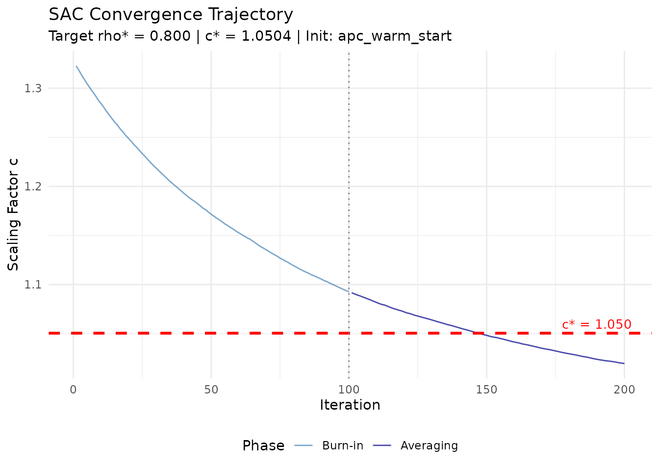

Line plot of SAC scaling factor iterates across stochastic approximation iterations.

SAC convergence trajectory (scaling factor).

plot(sac_res, type = "rho")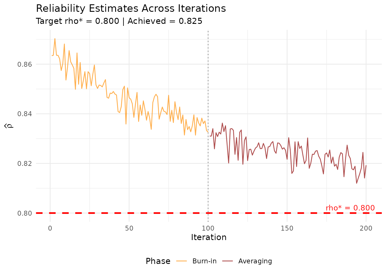

SAC reliability estimates across iterations.

4.3 Methods for `latent_G` Objects

Objects returned by sim_latentG().

`print.latent_G()`

print.latent_G(x, digits = 4, ...)

Prints shape, sample size, target parameters, and sample moments.

print(g_bimod)
#> Latent Ability Distribution (G-family)
#> =======================================
#>   Shape     : bimodal
#>   n         : 2000
#>   Target mu : 0.0000
#>   Target sigma: 1.0000
#> 
#> Sample Moments:
#>   Mean      : -0.0172
#>   SD        : 0.9885
#>   Skewness  : 0.0126
#>   Kurtosis  : -1.2981 (excess)

`summary.latent_G()`

summary.latent_G(object, ...)

Returns a "summary.latent_G" object with detailed statistics including quantiles.

summary(g_bimod)
#> Summary: Latent Ability Distribution
#> ====================================
#>   Shape      : bimodal
#>   n          : 2000
#>   Target     : mu = 0.00, sigma = 1.00
#>   Covariates : No
#> 
#> Sample Statistics:
#>   Mean       : -0.0172
#>   SD         : 0.9885
#>   Median     : -0.0657
#>   Skewness   : 0.0126
#>   Kurtosis   : -1.2981 (excess)
#>   Range      : [-2.2867, 2.4625]
#> 
#> Quantiles:
#>    2.5%      5%     25%     50%     75%     95%   97.5% 
#> -1.6338 -1.4650 -0.9025 -0.0657  0.8813  1.4319  1.5588

`plot.latent_G()`

plot.latent_G(x, type = c("both", "histogram", "density"),
              show_normal = TRUE, bins = 50, ...)

Plots the latent distribution as histogram, density, or both. Uses ggplot2 if available.

Parameter	Default	Description
`type`	`"both"`	Plot type: `"both"`, `"histogram"`, or `"density"`.
`show_normal`	`TRUE`	Overlay a normal reference density (dashed red).
`bins`	`50`	Number of histogram bins.

plot(g_bimod, type = "both", bins = 40)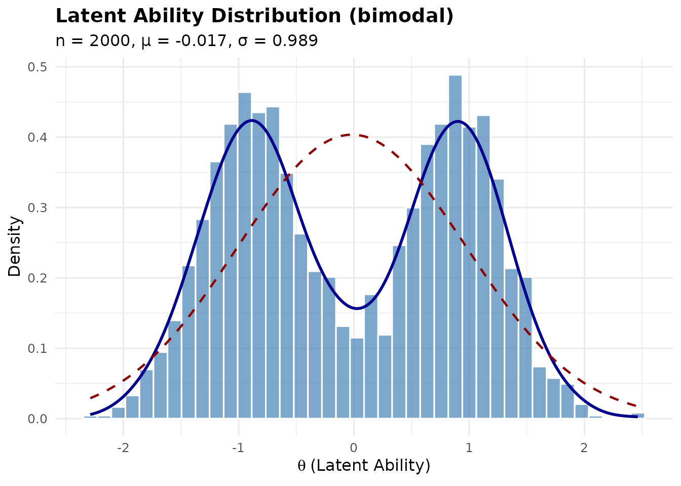

Bimodal latent ability distribution.

`as.numeric.latent_G()`

as.numeric.latent_G(x, ...)

Extracts the theta vector for use with other functions.

# Extract theta vector directly (equivalent to as.numeric dispatch)
theta_vec <- g_norm$theta
cat(sprintf("Length: %d, Mean: %.3f\n", length(theta_vec), mean(theta_vec)))
#> Length: 2000, Mean: -0.016

as.double() is registered as the same extraction path, so as.double(g_norm) also returns the stored theta vector.

4.4 Methods for `item_params` Objects

Objects returned by sim_item_params().

`print.item_params()`

print.item_params(x, digits = 4, ...)

Prints model, source, method, summary statistics of difficulties and discriminations, and achieved correlations.

print(items_2pl)
#> Item Parameters Object
#> ======================
#>   Model          : 2PL
#>   Source         : parametric
#>   Method         : copula
#>   Items per form : 30
#>   Number of forms: 1
#>   Scale factor   : 1.0000
#>   Centered       : Yes
#> 
#> Difficulty (beta):
#>   Mean: 0.0000, SD: 1.2550, Range: [-2.7250, 2.2181]
#> 
#> Discrimination (lambda, scaled):
#>   Mean: 1.0867, SD: 0.2885, Range: [0.4396, 1.7309]
#> 
#> Correlation (beta, log-lambda):
#>   Target (rho): -0.3000
#>   Achieved Pearson : -0.3611
#>   Achieved Spearman: -0.3784

`summary.item_params()`

summary.item_params(object, ...)

Returns a "summary.item_params" object with detailed parameter summaries.

summary(items_2pl)
#> Summary: Item Parameters
#> ========================
#>   Model          : 2PL
#>   Source         : parametric
#>   Method         : copula
#>   Items per form : 30
#>   Number of forms: 1
#>   Scale factor   : 1.000
#>   Centered       : Yes
#> 
#> Difficulty (beta):
#>   Mean     : 0.0000
#>   SD       : 1.2550
#>   Min      : -2.7250
#>   Max      : 2.2181
#>   Quantiles: Q25=-0.4681, Q50=-0.1690, Q75=1.0014
#> 
#> Discrimination (lambda):
#>   Before scaling: Mean=1.0867, SD=0.2885
#>   After scaling (c=1.000): Mean=1.0867, SD=0.2885
#>   Range [0.4396, 1.7309]
#> 
#> Correlation (beta, log-lambda):
#>   Target (rho)     : -0.3000
#>   Achieved Pearson : -0.3611
#>   Achieved Spearman: -0.3784

`plot.item_params()`

plot.item_params(x, type = c("scatter", "density", "both"), ...)

For 2PL and 3PL models, creates difficulty-versus-discrimination scatter plots and/or density plots; the 3PL density view also includes the guessing distribution. Rasch output uses the applicable difficulty/discrimination summaries. Uses ggplot2 if available.

Parameter	Default	Description
`type`	`"scatter"`	`"scatter"`, `"density"`, or `"both"`.

plot(items_2pl, type = "scatter")
#> `geom_smooth()` using formula = 'y ~ x'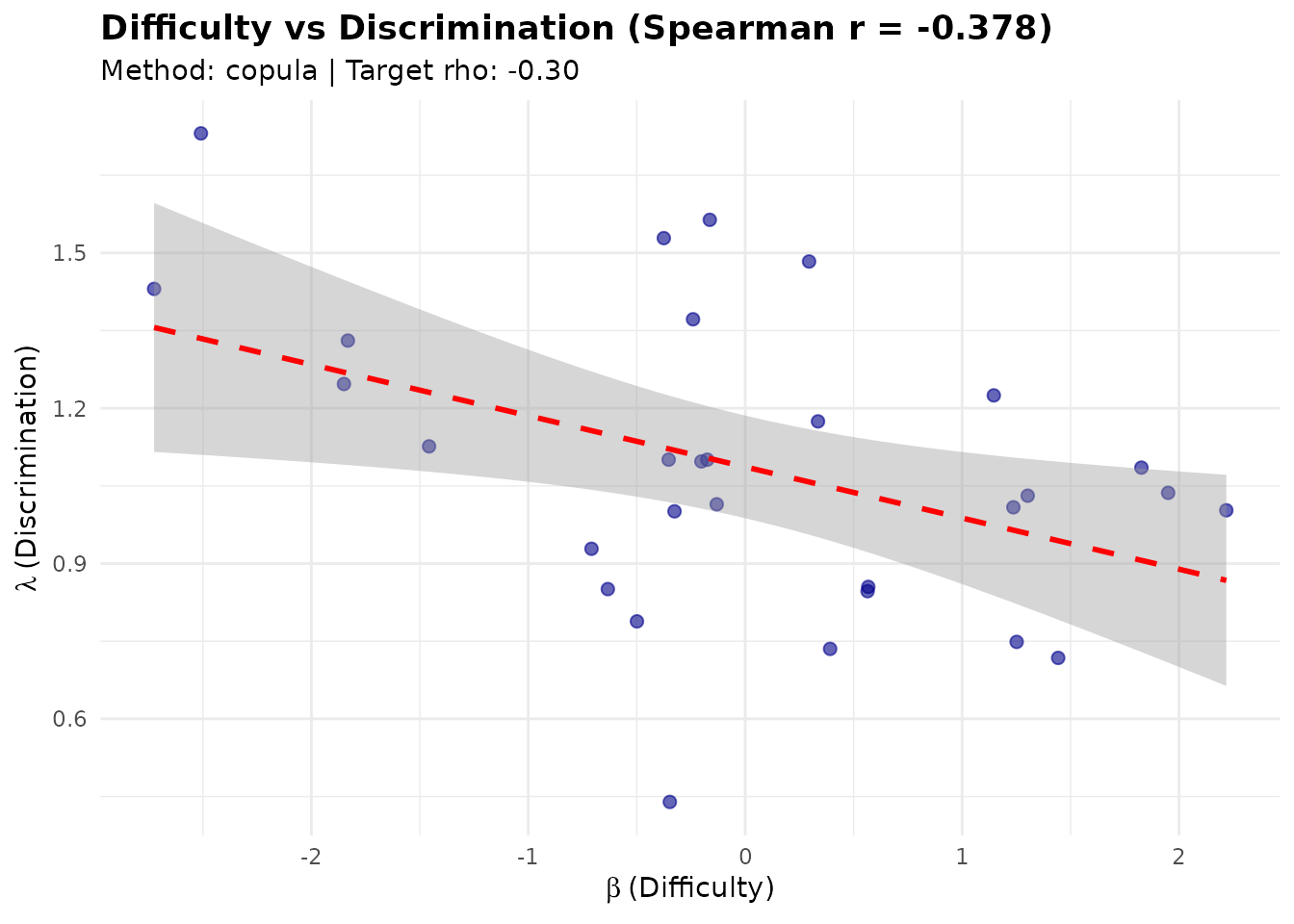

Scatter plot of item difficulty against scaled discrimination for a 2PL item set.

Difficulty vs. discrimination scatter plot.

`as.data.frame.item_params()`

as.data.frame.item_params(x, row.names = NULL, optional = FALSE, ...)

Extracts the item parameter data frame.

df <- as.data.frame(items_rasch)
head(df)
#>   form_id item_id       beta lambda lambda_unscaled
#> 1       1       1  1.1834223      1               1
#> 2       1       2 -0.7522343      1               1
#> 3       1       3  0.1755922      1               1
#> 4       1       4  0.4453264      1               1
#> 5       1       5  0.2167322      1               1
#> 6       1       6 -0.2936607      1               1

4.5 Methods for `feasibility_check` Objects

Objects returned by check_feasibility().

`print.feasibility_check()`

print.feasibility_check(x, digits = 4, ...)

Prints achievable reliability ranges and design information.

print(feas)
#> 
#> =======================================================
#>   Feasibility Check: Achievable Reliability Range
#> =======================================================
#> 
#>   Number of items  : 25
#>   Model            : RASCH
#>   Latent shape     : normal
#>   Latent variance  : 1.0099
#>   c range          : [0.10, 10.00]
#>   Monte Carlo M    : 5000
#> 
#> Achievable Reliability Ranges:
#>   rho_tilde (info) : [0.0591, 0.9872]
#>   rho_bar   (msem) : [0.0002, 0.9146]
#> 
#> Target rho*        : 0.8500
#>   info status      : feasible
#>   msem status      : feasible
#> 
#> Note: rho_tilde >= rho_bar on the same information grid (Jensen's inequality).
#>   rho_tilde range screens EQC targets; root policy must still admit a root.
#>   rho_bar range screens SAC targets; stable interior-branch preflight is also required.

4.6 Methods for `rho_curve` Objects

Objects returned by rho_curve().

`print.rho_curve()`

print.rho_curve(x, ...)

Prints a compact summary of the reliability curve data and the first few rows.

print(curve_data)
#> Reliability Curve
#> =================
#>   Items: 25 | Model: RASCH | Metric: both
#>   c range: [0.20, 4.00] (40 points)
#>   rho_tilde range: [0.1989, 0.9672]
#>   rho_bar range  : [0.1989, 0.9146]
#> 
#>           c rho_tilde   rho_bar
#> 1 0.2000000 0.1988965 0.1988657
#> 2 0.2974359 0.3500759 0.3498742
#> 3 0.3948718 0.4807284 0.4800963
#> 4 0.4923077 0.5827614 0.5814095
#> 5 0.5897436 0.6596796 0.6573608
#> 6 0.6871795 0.7174113 0.7139425
#>   ... (34 more rows)

4.7 Summary Print Methods

Each summary class has its own print method that displays formatted output.

`print.summary.eqc_result()`

print.summary.eqc_result(x, digits = 4, ...)

print(summary(eqc_res))
#> Summary: Empirical Quadrature Calibration (EQC)
#> ================================================
#>   Model            : RASCH
#>   Metric           : Average-information (tilde)
#>   Number of items  : 25
#>   Quadrature (M)   : 5000
#>   Latent variance  : 1.0099
#> 
#> Calibration Results:
#>   Target rho*      : 0.8000
#>   Achieved rho     : 0.8000
#>   Absolute error   : 4.64e-08
#>   Scaling factor c*: 0.8995
#>   Root status      : uniroot_success
#>   Calibration      : ok
#>   Roots detected   : 1

`print.summary.sac_result()`

print.summary.sac_result(x, digits = 4, ...)

print(summary(sac_res))
#> Summary: Stochastic Approximation Calibration (SAC)
#> ====================================================
#>   Model            : RASCH
#>   Metric           : MSEM-based (bar/w)
#>   Item scope       : item_superpopulation
#>   Number of items  : 25
#>   Iterations       : 200
#>   Burn-in          : 100
#>   M per iteration  : 500
#>   M pre-calc       : 5000
#>   Latent variance  : 1.0099
#>   Init method      : apc_warm_start
#> 
#> Calibration Results:
#>   Target rho*      : 0.8000
#>   Achieved rho     : 0.8250
#>   Achieved SE      : 0.0008
#>   Evaluation forms : 20
#>   Absolute error   : 2.50e-02
#>   Scaling factor c*: 1.0504
#>   Status           : ok
#>   Selected root    : 0.9530
#>   Selected branch  : id=1, increasing, [0.01, 2.52]
#>   Root policy      : lowest_increasing
#>   Converged        : Yes
#>   Post-burn-in SD  : 0.0210

`print.summary.item_params()`

print.summary.item_params(x, digits = 4, ...)

print(summary(items_2pl))
#> Summary: Item Parameters
#> ========================
#>   Model          : 2PL
#>   Source         : parametric
#>   Method         : copula
#>   Items per form : 30
#>   Number of forms: 1
#>   Scale factor   : 1.000
#>   Centered       : Yes
#> 
#> Difficulty (beta):
#>   Mean     : 0.0000
#>   SD       : 1.2550
#>   Min      : -2.7250
#>   Max      : 2.2181
#>   Quantiles: Q25=-0.4681, Q50=-0.1690, Q75=1.0014
#> 
#> Discrimination (lambda):
#>   Before scaling: Mean=1.0867, SD=0.2885
#>   After scaling (c=1.000): Mean=1.0867, SD=0.2885
#>   Range [0.4396, 1.7309]
#> 
#> Correlation (beta, log-lambda):
#>   Target (rho)     : -0.3000
#>   Achieved Pearson : -0.3611
#>   Achieved Spearman: -0.3784

`print.summary.latent_G()`

print.summary.latent_G(x, digits = 4, ...)

print(summary(g_norm))
#> Summary: Latent Ability Distribution
#> ====================================
#>   Shape      : normal
#>   n          : 2000
#>   Target     : mu = 0.00, sigma = 1.00
#>   Covariates : No
#> 
#> Sample Statistics:
#>   Mean       : -0.0156
#>   SD         : 0.9941
#>   Median     : -0.0131
#>   Skewness   : 0.0128
#>   Kurtosis   : 0.0560 (excess)
#>   Range      : [-3.3717, 3.5847]
#> 
#> Quantiles:
#>    2.5%      5%     25%     50%     75%     95%   97.5% 
#> -1.9835 -1.6446 -0.6691 -0.0131  0.6608  1.5768  1.8871

5. Deprecated Functions

These functions are retained for backward compatibility and will be removed in a future release. They issue a deprecation warning when called.

5.1 `spc_calibrate()`

spc_calibrate(...)

Deprecated alias for sac_calibrate(). All arguments are passed through unchanged. Use sac_calibrate() for new code.

# Deprecated: use sac_calibrate() instead
result <- spc_calibrate(
  target_rho = 0.80, n_items = 25, model = "rasch",
  n_iter = 200, seed = 42
)

5.2 `compare_eqc_spc()`

compare_eqc_spc(...)

Deprecated alias for compare_eqc_sac(). All arguments are passed through unchanged. Use compare_eqc_sac() for new code.

# Deprecated: use compare_eqc_sac() instead
compare_eqc_spc(eqc_res, sac_warm)

6. Cross-Reference Table

The table below maps each function to the vignette that covers it in detail.

Function	Category	Primary Vignette
`eqc_calibrate()`	Calibration	`vignette("algorithm-eqc")`
`sac_calibrate()`	Calibration	`vignette("algorithm-sac")`
`compare_eqc_sac()`	Calibration	`vignette("applied-guide")`
`sim_latentG()`	Simulation	`vignette("latent-distributions")`
`compare_shapes()`	Simulation	`vignette("latent-distributions")`
`sim_item_params()`	Simulation	`vignette("item-parameters")`
`simulate_response_data()`	Simulation	`vignette("applied-guide")`
`compute_rho_bar()`	Reliability	`vignette("theory-reliability")`
`compute_rho_tilde()`	Reliability	`vignette("theory-reliability")`
`compute_rho_both()`	Reliability	`vignette("theory-reliability")`
`compute_apc_init()`	Reliability	`vignette("algorithm-sac")`
`check_feasibility()`	Reliability	`vignette("simulation-design")`
`rho_curve()`	Reliability	`vignette("simulation-design")`
`compute_reliability_tam()`	Validation	`vignette("validation")`
`spc_calibrate()`	Deprecated	–
`compare_eqc_spc()`	Deprecated	–

7. Complete Workflow Example

This section demonstrates a full simulation study using the IRTsimrel API.

Step 1: Check Feasibility

feas_check <- check_feasibility(
  n_items    = 30,
  model      = "rasch",
  M          = 5000L,
  target_rho = 0.85,
  seed       = 42,
  verbose    = FALSE
)
cat(sprintf("For 30 Rasch items, achievable rho_tilde: [%.3f, %.3f]\n",
            feas_check$rho_range_info[1], feas_check$rho_range_info[2]))
#> For 30 Rasch items, achievable rho_tilde: [0.070, 0.989]
cat(sprintf("Target status (info): %s\n",
            feas_check$target_status_info))
#> Target status (info): feasible

Step 2: Calibrate with EQC

eqc_wf <- eqc_calibrate(
  target_rho = 0.85,
  n_items    = 30,
  model      = "rasch",
  reliability_metric = "info",
  M          = 5000L,
  seed       = 42
)
cat(sprintf("EQC: c* = %.4f, rho = %.4f\n",
            eqc_wf$c_star, eqc_wf$achieved_rho))
#> EQC: c* = 0.9943, rho = 0.8500

Step 3: Validate with SAC

sac_wf <- sac_calibrate(
  target_rho = 0.85,
  n_items    = 30,
  model      = "rasch",
  reliability_metric = "info",
  c_init     = eqc_wf,
  resample_items = FALSE,
  n_iter     = 150L,
  M_per_iter = 500L,
  M_pre      = 5000L,
  seed       = 42,
  verbose    = FALSE
)
cat(sprintf("SAC: c* = %.4f, rho = %.4f\n",
            sac_wf$c_star, sac_wf$achieved_rho))
#> SAC: c* = 0.9943, rho = 0.8501

Step 4: Compare Results

comp_wf <- compare_eqc_sac(eqc_wf, sac_wf, verbose = TRUE)
#> 
#> =======================================================
#>   EQC vs SAC Comparison
#> =======================================================
#> 
#>   Target reliability  : 0.8500
#>   EQC c*              : 0.994328
#>   SAC c*              : 0.994341
#>   Absolute difference : 0.000012
#>   Percent difference  : 0.00%
#>   EQC achieved rho    : 0.8500
#>   SAC achieved rho    : 0.8501
#>   Comparable           : YES
#>   Agreement (< 5%)    : YES
#>   Agreement status     : evaluated
#>   EQC status          : uniroot_success
#>   SAC status          : ok
#>   SAC status flags    : ok
#>

Step 5: Generate Response Data

resp_wf <- simulate_response_data(
  result    = eqc_wf,
  n_persons = 1000,
  seed      = 123
)
cat(sprintf("Generated %d x %d response matrix\n",
            nrow(resp_wf$response_matrix),
            ncol(resp_wf$response_matrix)))
#> Generated 1000 x 30 response matrix
cat(sprintf("Mean score: %.2f / %d items\n",
            mean(rowSums(resp_wf$response_matrix)),
            ncol(resp_wf$response_matrix)))
#> Mean score: 15.00 / 30 items
resp_wf$provenance[c("metric", "calibration_status", "simulation_seed")]
#> $metric
#> [1] "info"
#> 
#> $calibration_status
#> [1] "uniroot_success"
#> 
#> $simulation_seed
#> [1] 123

Step 6: Extract Calibrated Parameters

params_wf <- coef(eqc_wf)
head(params_wf)
#>   item_id        beta lambda_base lambda_scaled    c_star
#> 1       1  0.17744288           1     0.9943282 0.9943282
#> 2       2  1.07651047           1     0.9943282 0.9943282
#> 3       3  0.41625569           1     0.9943282 0.9943282
#> 4       4 -0.03332812           1     0.9943282 0.9943282
#> 5       5 -0.22009069           1     0.9943282 0.9943282
#> 6       6 -0.01258907           1     0.9943282 0.9943282
cat(sprintf("\nScaled discrimination: mean = %.3f, sd = %.3f\n",
            mean(params_wf$lambda_scaled),
            sd(params_wf$lambda_scaled)))
#> 
#> Scaled discrimination: mean = 0.994, sd = 0.000

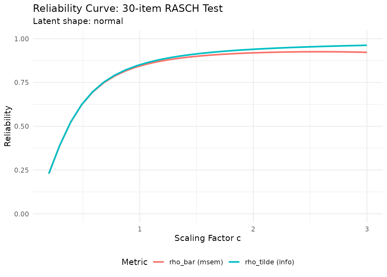
Step 7: Explore Reliability Curve

rc_wf <- rho_curve(
  c_values = seq(0.2, 3, length.out = 30),
  n_items  = 30,
  model    = "rasch",
  M        = 5000L,
  seed     = 42,
  plot     = TRUE
)

Reliability curve across scaling factors for the complete workflow example.

Reliability curve for the workflow example.

Step 8: Validate with TAM (optional)

if (requireNamespace("TAM", quietly = TRUE)) {
  tam_wf <- compute_reliability_tam(
    resp  = resp_wf$response_matrix,
    model = "rasch"
  )
  cat(sprintf("WLE reliability: %.4f\n", tam_wf$rel_wle))
  cat(sprintf("EAP reliability: %.4f\n", tam_wf$rel_eap))
  cat(sprintf("Target reliability: %.4f\n", eqc_wf$target_rho))
}

8. Exported Functions and Registered S3 Methods

The table below lists the user-facing functions exported by IRTsimrel plus registered S3 methods from the NAMESPACE file, organized alphabetically.

Export	Type
`as.data.frame.item_params`	S3 method
`as.double.latent_G`	S3 method
`as.numeric.latent_G`	S3 method
`check_feasibility`	Function
`coef.eqc_result`	S3 method
`coef.sac_result`	S3 method
`compare_eqc_sac`	Function
`compare_eqc_spc`	Function (deprecated)
`compare_shapes`	Function
`compute_apc_init`	Function
`compute_reliability_tam`	Function
`compute_rho_bar`	Function
`compute_rho_both`	Function
`compute_rho_tilde`	Function
`eqc_calibrate`	Function
`plot.item_params`	S3 method
`plot.latent_G`	S3 method
`plot.sac_result`	S3 method
`predict.eqc_result`	S3 method
`predict.sac_result`	S3 method
`print.eqc_result`	S3 method
`print.feasibility_check`	S3 method
`print.item_params`	S3 method
`print.latent_G`	S3 method
`print.rho_curve`	S3 method
`print.sac_result`	S3 method
`print.summary.eqc_result`	S3 method
`print.summary.item_params`	S3 method
`print.summary.latent_G`	S3 method
`print.summary.sac_result`	S3 method
`rho_curve`	Function
`sac_calibrate`	Function
`sim_item_params`	Function
`sim_latentG`	Function
`simulate_response_data`	Function
`spc_calibrate`	Function (deprecated)
`summary.eqc_result`	S3 method
`summary.item_params`	S3 method
`summary.latent_G`	S3 method
`summary.sac_result`	S3 method

Session Information

sessionInfo()
#> R version 4.6.1 (2026-06-24)
#> Platform: x86_64-pc-linux-gnu
#> Running under: Ubuntu 24.04.4 LTS
#> 
#> Matrix products: default
#> BLAS:   /usr/lib/x86_64-linux-gnu/openblas-pthread/libblas.so.3 
#> LAPACK: /usr/lib/x86_64-linux-gnu/openblas-pthread/libopenblasp-r0.3.26.so;  LAPACK version 3.12.0
#> 
#> locale:
#>  [1] LC_CTYPE=C.UTF-8       LC_NUMERIC=C           LC_TIME=C.UTF-8       
#>  [4] LC_COLLATE=C.UTF-8     LC_MONETARY=C.UTF-8    LC_MESSAGES=C.UTF-8   
#>  [7] LC_PAPER=C.UTF-8       LC_NAME=C              LC_ADDRESS=C          
#> [10] LC_TELEPHONE=C         LC_MEASUREMENT=C.UTF-8 LC_IDENTIFICATION=C   
#> 
#> time zone: UTC
#> tzcode source: system (glibc)
#> 
#> attached base packages:
#> [1] stats     graphics  grDevices utils     datasets  methods   base     
#> 
#> other attached packages:
#> [1] IRTsimrel_0.3.0
#> 
#> loaded via a namespace (and not attached):
#>  [1] vctrs_0.7.3        nlme_3.1-169       cli_3.6.6          knitr_1.51        
#>  [5] rlang_1.3.0        xfun_0.60          otel_0.2.0         textshaping_1.0.5 
#>  [9] S7_0.2.2           jsonlite_2.0.0     labeling_0.4.3     glue_1.8.1        
#> [13] htmltools_0.5.9    ragg_1.5.2         sass_0.4.10        scales_1.4.0      
#> [17] rmarkdown_2.31     grid_4.6.1         evaluate_1.0.5     jquerylib_0.1.4   
#> [21] MASS_7.3-65        fastmap_1.2.0      yaml_2.3.12        lifecycle_1.0.5   
#> [25] compiler_4.6.1     fs_2.1.0           RColorBrewer_1.1-3 mgcv_1.9-4        
#> [29] lattice_0.22-9     systemfonts_1.3.2  farver_2.1.2       digest_0.6.39     
#> [33] R6_2.6.1           splines_4.6.1      Matrix_1.7-5       bslib_0.12.0      
#> [37] withr_3.0.3        tools_4.6.1        gtable_0.3.6       pkgdown_2.2.1     
#> [41] ggplot2_4.0.3      cachem_1.1.0       desc_1.4.3

JoonHo Lee (jlee296@ua.edu)

2026-08-22

Overview

1. Calibration Functions

1.1 eqc_calibrate() – Empirical Quadrature Calibration

Signature

Parameters

Return Value

Examples

1.2 sac_calibrate() – Stochastic Approximation Calibration

Signature

Parameters

Return Value

Examples

1.3 compare_eqc_sac() – Compare Calibration Results

Signature

Parameters

Return Value

Examples

2. Simulation Functions

2.1 sim_latentG() – Simulate Latent Ability Distributions

Signature

Parameters

Return Value

Examples

2.2 sim_item_params() – Simulate Item Parameters

Signature

Parameters

Return Value

Examples

2.3 simulate_response_data() – Generate Response Matrices

Signature

Parameters

Return Value

Examples

2.4 compare_shapes() – Compare Distribution Shapes

Signature

Parameters

Return Value

Example

3. Reliability Functions

3.1 compute_rho_bar() – MSEM-Based Marginal Reliability

Signature

Parameters

Return Value

Example

3.2 compute_rho_tilde() – Average-Information Reliability

Signature

Example

3.3 compute_rho_both() – Both Metrics in a Single Pass

Signature

Return Value

Example

3.4 compute_apc_init() – Analytic Pre-Calibration

Signature

Parameters

Return Value

Example

3.5 check_feasibility() – Feasibility Screening

Signature

Parameters

Return Value

Example

3.6 rho_curve() – Reliability as a Function of Scaling Factor

Signature

Parameters

Return Value

Example

3.7 compute_reliability_tam() – TAM-Based Validation

Signature

Parameters

Return Value

Example

4. S3 Methods

4.1 Methods for eqc_result Objects

print.eqc_result()

summary.eqc_result()

coef.eqc_result()

predict.eqc_result()

1.1 `eqc_calibrate()` – Empirical Quadrature Calibration

1.2 `sac_calibrate()` – Stochastic Approximation Calibration

1.3 `compare_eqc_sac()` – Compare Calibration Results

2.1 `sim_latentG()` – Simulate Latent Ability Distributions

2.2 `sim_item_params()` – Simulate Item Parameters

2.3 `simulate_response_data()` – Generate Response Matrices

2.4 `compare_shapes()` – Compare Distribution Shapes

3.1 `compute_rho_bar()` – MSEM-Based Marginal Reliability

3.2 `compute_rho_tilde()` – Average-Information Reliability

3.3 `compute_rho_both()` – Both Metrics in a Single Pass

3.4 `compute_apc_init()` – Analytic Pre-Calibration

3.5 `check_feasibility()` – Feasibility Screening

3.6 `rho_curve()` – Reliability as a Function of Scaling Factor

3.7 `compute_reliability_tam()` – TAM-Based Validation

4.1 Methods for `eqc_result` Objects

`print.eqc_result()`

`summary.eqc_result()`

`coef.eqc_result()`

`predict.eqc_result()`

4.2 Methods for `sac_result` Objects

`print.sac_result()`

`summary.sac_result()`

`coef.sac_result()`

`predict.sac_result()`

`plot.sac_result()`

4.3 Methods for `latent_G` Objects

`print.latent_G()`

`summary.latent_G()`

`plot.latent_G()`

`as.numeric.latent_G()`

4.4 Methods for `item_params` Objects

`print.item_params()`

`summary.item_params()`

`plot.item_params()`

`as.data.frame.item_params()`

4.5 Methods for `feasibility_check` Objects

`print.feasibility_check()`

4.6 Methods for `rho_curve` Objects

`print.rho_curve()`

`print.summary.eqc_result()`

`print.summary.sac_result()`

`print.summary.item_params()`

`print.summary.latent_G()`

5.1 `spc_calibrate()`

5.2 `compare_eqc_spc()`