Algorithm 2: Stochastic Approximation Calibration (SAC)

JoonHo Lee (jlee296@ua.edu)

2026-08-22

library(IRTsimrel)
set.seed(42)

Overview

Stochastic Approximation Calibration (SAC) is the secondary algorithm in IRTsimrel, designed to complement EQC (Algorithm 1). SAC uses the Robbins-Monro stochastic approximation framework to find the discrimination scaling factor c^* that achieves a target reliability.

Reading time: approximately 25 minutes.

Positioning: SAC serves both as the direct MSEM-targeting algorithm and as a validation companion to EQC. When validating EQC, set reliability_metric = "info" so both algorithms target the same estimand. SAC also provides trajectory-based convergence diagnostics that EQC lacks.

Prerequisites: Familiarity with vignette("theory-reliability") for the mathematical foundations. For applied workflows, see vignette("introduction").

Key references: Lee (2026, arXiv:2512.16012v2), Section 2.5; Robbins and Monro (1951); Polyak and Juditsky (1992); Kushner and Yin (2003).

When to Use SAC

Use Case	Recommendation
Routine simulation studies	Use EQC (faster, no tuning)
Independent validation of EQC	Use SAC with EQC warm start and reliability_metric = "info"
Direct MSEM targeting	Use SAC with reliability_metric = "msem"
Convergence diagnostics	SAC provides trajectory plots
Research on stochastic approximation	Use SAC

The built-in Student-t heavy_tail population is not compatible with population MSEM targeting: its reciprocal-information expectation diverges. SAC rejects that combination before iteration. Use the information metric or define and label an explicitly truncated empirical design.

Item scope is part of the target

resample_items = FALSE defines a fixed-form target. The same realized item bank is used in preflight, every stochastic update, and independent theta evaluation. resample_items = TRUE defines an item-superpopulation target: fresh forms are drawn during calibration and achieved_rho is the mean of form-level reliabilities over an independent evaluation bank. It is not the reliability obtained by pooling information across forms. Result fields item_scope, estimand_signature, and achieved_distribution make the distinction explicit.

For model = "3pl", lower asymptotes are supplied through item_params$guessing_params and remain fixed within each item form while the global scale multiplies discrimination only. The result stores guessing_vec; coef() appends a guessing column only for 3PL results. All-zero guessing follows the 2PL numerical path exactly. The letter c below always denotes the global discrimination scale, never the 3PL lower asymptote.

The Robbins-Monro Framework

The Stochastic Root-Finding Problem

After deterministic branch preflight, SAC uses stochastic approximation to solve:

g(c) = \mathbb{E}\!\left[\hat{\rho}(c)\right] - \rho^* = 0 \qquad \text{(1)}

where g(c) = \rho(c) - \rho^* is the reliability gap function. At each iteration n, it observes a noisy evaluation:

Y_n = \hat{\rho}_n(c_n) = \rho(c_n) + \varepsilon_n \qquad \text{(2)}

where \hat{\rho}_n is computed from fresh theta samples at each step (and fresh item forms only for the item-superpopulation scope), and \varepsilon_n is zero-mean noise with bounded variance: \mathbb{E}[\varepsilon_n \mid c_n] = 0 and \mathbb{E}[\varepsilon_n^2 \mid c_n] \leq \sigma^2_\varepsilon.

Branch preflight

Before the first update, SAC evaluates a common-random-number pilot bank over the configured log-scale interval. It requires a resolved, feasible, interior increasing crossing and narrows projection bounds to that selected branch. For item-superpopulation calibration, two disjoint form splits must select compatible roots with overlapping branch intervals. Infeasible, decreasing, boundary-only, non-finite, resolution-limited, or split-unstable cases stop with an irtsimrel_sac_* classed error. The preflight bank is isolated from the iteration and evaluation RNG streams.

The Robbins-Monro Update Rule

The iterative update proceeds as:

c_{n+1} = \Pi_{[c_L, c_U]}\!\left[c_n - a_n\,(\hat{\rho}_n(c_n) - \rho^*)\right] \qquad \text{(3)}

where \Pi_{[c_L, c_U]}[\cdot] denotes projection onto the effective interior of the selected branch (itself contained in the user bounds) and a_n is a decreasing step size sequence.

Intuition: When \hat{\rho}_n(c_n) > \rho^* (current reliability is too high), the update decreases c_n (reducing discrimination, hence reliability). When \hat{\rho}_n(c_n) < \rho^*, the update increases c_n.

Robbins-Monro Conditions

The step size sequence must satisfy:

\sum_{n=1}^{\infty} a_n = \infty \quad\text{and}\quad \sum_{n=1}^{\infty} a_n^2 < \infty \qquad \text{(4)}

First condition (\Sigma a_n = \infty): Ensures the algorithm can reach any point in the parameter space, regardless of the initial value. Without this, the total adjustment \sum a_n \cdot |\hat{\rho}_n - \rho^*| might be bounded, preventing convergence from a distant starting point.

Second condition (\Sigma a_n^2 < \infty): Controls the accumulated noise. The total noise variance is proportional to \sum a_n^2 \sigma^2_\varepsilon, which must be finite for convergence.

Step Size Analysis

The Step Size Sequence

SAC uses the parametric family:

a_n = \frac{a}{(n + A)^\gamma} \qquad \text{(5)}

with three parameters controlling different aspects of the learning dynamics.

Role of Each Parameter

a > 0 (scale constant): Controls the overall magnitude of updates. Larger a means more aggressive steps, leading to faster initial progress but potentially more oscillation.

In the package: step_params$a (default: 1).

A \geq 0 (stabilization constant): Dampens early iterations where step sizes would otherwise be very large (a_1 = a/(1+A)^\gamma). When A > 0, the effective step size starts smaller, providing stability during the initial transient phase. This is particularly important when c_init is far from c^*.

In the package, step_params$A defaults to 50. The burn_in argument controls which iterations enter the Polyak-Ruppert average; it does not set A automatically.

\gamma \in (1/2, 1] (decay exponent): Controls how quickly step sizes decrease. In the package: step_params$gamma (default: 0.67).

• \gamma = 0.51: Slow decay, close to the boundary of the Robbins-Monro conditions. Maintains larger steps for longer, which can be beneficial when initial estimates are poor.
• \gamma = 2/3: A common compromise between convergence speed and stability.
• \gamma = 1: Fastest allowable decay. Reduces variance quickly but may under-correct if the initial value is far from the solution.

Robbins-Monro Conditions Verification

For the parametric family a_n = a/(n+A)^\gamma:

\sum_{n=1}^{\infty} \frac{a}{(n+A)^\gamma} = \infty \quad\iff\quad \gamma \leq 1

\sum_{n=1}^{\infty} \frac{a^2}{(n+A)^{2\gamma}} < \infty \quad\iff\quad 2\gamma > 1 \;\iff\; \gamma > 1/2

Therefore, any \gamma \in (1/2, 1] satisfies both conditions.

Step Size Sensitivity

The effect of different step size configurations can be observed through the convergence trajectory.

# Common setup
eqc_ref <- eqc_calibrate(
  target_rho = 0.80, n_items = 25, model = "rasch",
  item_source = "parametric", M = 5000L, seed = 42, verbose = FALSE
)

# Run SAC with different step decay values
decays <- c(0.51, 0.67, 0.85, 1.0)
colors <- c("steelblue", "coral", "seagreen", "purple")

oldpar <- par(mar = c(4.5, 4.5, 3, 1))
on.exit(par(oldpar))

plot(NULL, xlim = c(1, 300), ylim = c(0.5, 2.5),
     xlab = "Iteration", ylab = "c_n",
     main = "SAC Trajectories: Step Decay Sensitivity")
abline(h = eqc_ref$c_star, lty = 2, col = "gray40", lwd = 1.5)

for (k in seq_along(decays)) {
  sac_k <- sac_calibrate(
    target_rho = 0.80, n_items = 25, model = "rasch",
    item_source = "parametric", reliability_metric = "info",
    c_init = 0.5,  # deliberately poor start
    n_iter = 300L, M_per_iter = 1000L,
    step_params = list(gamma = decays[k]),
    seed = 42, verbose = FALSE
  )
  lines(seq_along(sac_k$trajectory), sac_k$trajectory,
        col = colors[k], lwd = 1.5)
}
#> Warning: SAC may not have fully converged (status: not_converged; achieved gap:
#> -0.0748).

legend("topright",
       legend = c(sprintf("gamma = %.2f", decays), "EQC c*"),
       col = c(colors, "gray40"), lty = c(rep(1, 4), 2),
       lwd = c(rep(1.5, 4), 1.5), cex = 0.85)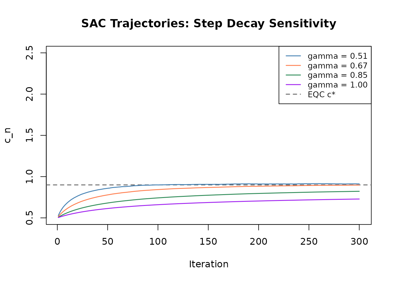

Effect of step decay parameter on SAC convergence trajectories.

Observations:

• Slower decay (\gamma = 0.51) maintains larger oscillations longer but eventually converges.
• Faster decay (\gamma = 1.0) converges quickly when starting near the solution, but risks under-correcting from a distant start.
• The default \gamma = 0.67 provides a good compromise between speed and stability.

Polyak-Ruppert Averaging

Why Averaging?

Under the usual locally linear stochastic-approximation conditions, a last iterate with step size n^{-\gamma} typically has mean-squared error of order n^{-\gamma}. Polyak and Juditsky (1992) showed that averaging can attain the optimal n^{-1} mean-squared-error order, equivalently an n^{-1/2} error scale, under the additional regularity conditions of the CLT.

The Averaging Formula

After discarding a burn-in period of B iterations, the Polyak-Ruppert average is:

\bar{c}_N = \frac{1}{N - B} \sum_{n=B+1}^{N} c_n \qquad \text{(6)}

where N is the total number of iterations and B is the burn-in count.

Convergence Rate Comparison

Estimator	Error scale	MSE order	Notes
Final iterate c_N	typically O_p(N^{-\gamma/2})	O(N^{-\gamma})	Depends on step schedule and local conditions
Polyak-Ruppert \bar{c}_N	O_p(N^{-1/2})	O(N^{-1})	Optimal under the stated averaging CLT
Truncated average	O_p(N^{-1/2})	O(N^{-1})	Requires an admissible burn-in sequence

With \gamma = 0.67 (the package default), this heuristic comparison gives a last-iterate error scale near n^{-0.335} versus the averaged n^{-0.5} scale. These are asymptotic orders under local assumptions, not finite-run guarantees for every IRT reliability curve.

Burn-In Selection

The burn-in period B should be large enough to exclude the initial transient (before the iterates have approached the solution) but small enough to include a sufficient number of post-burn-in samples.

In the package: burn_in parameter, specified as an integer count (default: floor(n_iter / 2), i.e., 50% of iterations).

Guidelines:

• With EQC warm start: the default burn_in = floor(n_iter / 2) is sufficient (starting near the solution, transient is short).
• With cold start or APC: the default 50% burn-in is appropriate; for very long runs (N > 1000), a smaller fraction (e.g., burn_in = floor(n_iter / 5)) can be used to include more post-burn-in samples.

Initialization Strategies

The initial value c_0 significantly affects SAC’s convergence speed. The package supports three initialization methods.

Strategy 1: EQC Warm Start (Recommended)

Pass an eqc_result object directly to c_init:

An EQC object is accepted only for the same target, model, item count, metric, and fixed-form scope. Leave item_source and item_params unspecified so SAC can reuse the stored EQC form exactly. Supplying an EQC-info result to initialize an MSEM run is a contract mismatch; use a numeric scale when the initializer is only a heuristic and label the designs separately.

eqc_for_init <- eqc_calibrate(
  target_rho = 0.80, n_items = 25, model = "rasch",
  item_source = "parametric", M = 5000L, seed = 42, verbose = FALSE
)

fixed_rasch_init <- list(
  custom_params = list(
    beta = eqc_for_init$beta_vec,
    lambda = eqc_for_init$lambda_base
  ),
  center_difficulties = FALSE
)

sac_warm <- sac_calibrate(
  target_rho = 0.80, n_items = 25, model = "rasch",
  reliability_metric = "info", resample_items = FALSE,
  c_init = eqc_for_init,  # EQC warm start
  n_iter = 200L, M_per_iter = 1000L,
  seed = 42, verbose = FALSE,
  preflight_controls = list(M = 500L),
  evaluation_controls = list(n_forms = 3L, M = 1000L)
)

cat(sprintf("EQC c*: %.4f\n", eqc_for_init$c_star))
#> EQC c*: 0.8995
cat(sprintf("SAC c* (warm start): %.4f\n", sac_warm$c_star))
#> SAC c* (warm start): 0.8982
cat(sprintf("Init method: %s\n", sac_warm$init_method))
#> Init method: eqc_warm_start

Advantages: Starting near the solution means the transient phase is short, burn-in can be minimal, and fewer iterations are needed.

Strategy 2: Analytic Pre-Calibration (APC)

When c_init = NULL, Rasch/2PL SAC first considers a closed-form approximation derived under Gaussian Rasch assumptions. If it lies outside the admissible preflight branch, the selected preflight root is used instead. For 3PL, APC is not a valid approximation and the selected preflight root is the default initializer.

Definition (APC Formula). Under the assumptions \theta \sim N(0, 1) and \beta_i \sim N(0, \sigma^2_\beta) with \lambda_i^{(0)} = 1 (Rasch), the approximate initial value is:

c_{\text{APC}} = \sqrt{\frac{\rho^*}{I \cdot \kappa(\sigma^2) \cdot (1 - \rho^*)}} \qquad \text{(7)}

where \sigma^2 = 1 + \sigma^2_\beta and the logistic-normal convolution constant is approximated by:

\kappa(\sigma^2) \approx \frac{0.25}{\sqrt{1 + \sigma^2 \pi^2 / 3}} \qquad \text{(8)}

Derivation sketch: Under the Gaussian Rasch model, the expected item information at a single item is \mathbb{E}[\lambda^2 p(1-p)] = c^2 \kappa(\sigma^2). With I items, the average test information is approximately I c^2 \kappa, so \tilde{\rho} \approx \sigma^2_\theta I c^2 \kappa / (\sigma^2_\theta I c^2 \kappa + 1). Setting this equal to \rho^* and solving for c yields Eq. (7).

# APC initialization (c_init = NULL triggers APC)
sac_apc <- sac_calibrate(
  target_rho = 0.80, n_items = 25, model = "rasch",
  item_source = "custom", item_params = fixed_rasch_init,
  reliability_metric = "info", resample_items = FALSE,
  c_init = NULL,  # APC warm start
  n_iter = 300L, M_per_iter = 1000L,
  seed = 42, verbose = FALSE,
  preflight_controls = list(M = 500L),
  evaluation_controls = list(n_forms = 3L, M = 1000L)
)

cat(sprintf("SAC c* (APC start): %.4f\n", sac_apc$c_star))
#> SAC c* (APC start): 0.9618
cat(sprintf("Init method: %s\n", sac_apc$init_method))
#> Init method: apc_warm_start

# Compare APC init quality
c_apc <- compute_apc_init(target_rho = 0.80, n_items = 25)
cat(sprintf("APC initial value: %.4f (vs true c* ~ %.4f)\n",
            c_apc, eqc_for_init$c_star))
#> APC initial value: 1.3274 (vs true c* ~ 0.8995)

Strategy 3: User-Specified Value

A numeric value can be passed directly:

sac_user <- sac_calibrate(
  target_rho = 0.80, n_items = 25, model = "rasch",
  item_source = "custom", item_params = fixed_rasch_init,
  reliability_metric = "info", resample_items = FALSE,
  c_init = 1.0,  # user-specified
  n_iter = 300L, M_per_iter = 1000L,
  seed = 42, verbose = FALSE,
  preflight_controls = list(M = 500L),
  evaluation_controls = list(n_forms = 3L, M = 1000L)
)

cat(sprintf("SAC c* (user init = 1.0): %.4f\n", sac_user$c_star))
#> SAC c* (user init = 1.0): 0.9086
cat(sprintf("Init method: %s\n", sac_user$init_method))
#> Init method: user_specified

Initialization Comparison

oldpar <- par(mar = c(4.5, 4.5, 3, 1))
on.exit(par(oldpar))

plot(NULL, xlim = c(1, 300), ylim = c(0, 3),
     xlab = "Iteration", ylab = "c_n",
     main = "Effect of Initialization on Convergence")
abline(h = eqc_for_init$c_star, lty = 2, col = "gray40", lwd = 1.5)

lines(seq_along(sac_warm$trajectory), sac_warm$trajectory,
      col = "steelblue", lwd = 1.5)
lines(seq_along(sac_apc$trajectory), sac_apc$trajectory,
      col = "coral", lwd = 1.5)
lines(seq_along(sac_user$trajectory), sac_user$trajectory,
      col = "seagreen", lwd = 1.5)

legend("topright",
       legend = c("EQC warm start", "APC", "User (c=1.0)", "EQC c*"),
       col = c("steelblue", "coral", "seagreen", "gray40"),
       lty = c(1, 1, 1, 2), lwd = 1.5, cex = 0.9)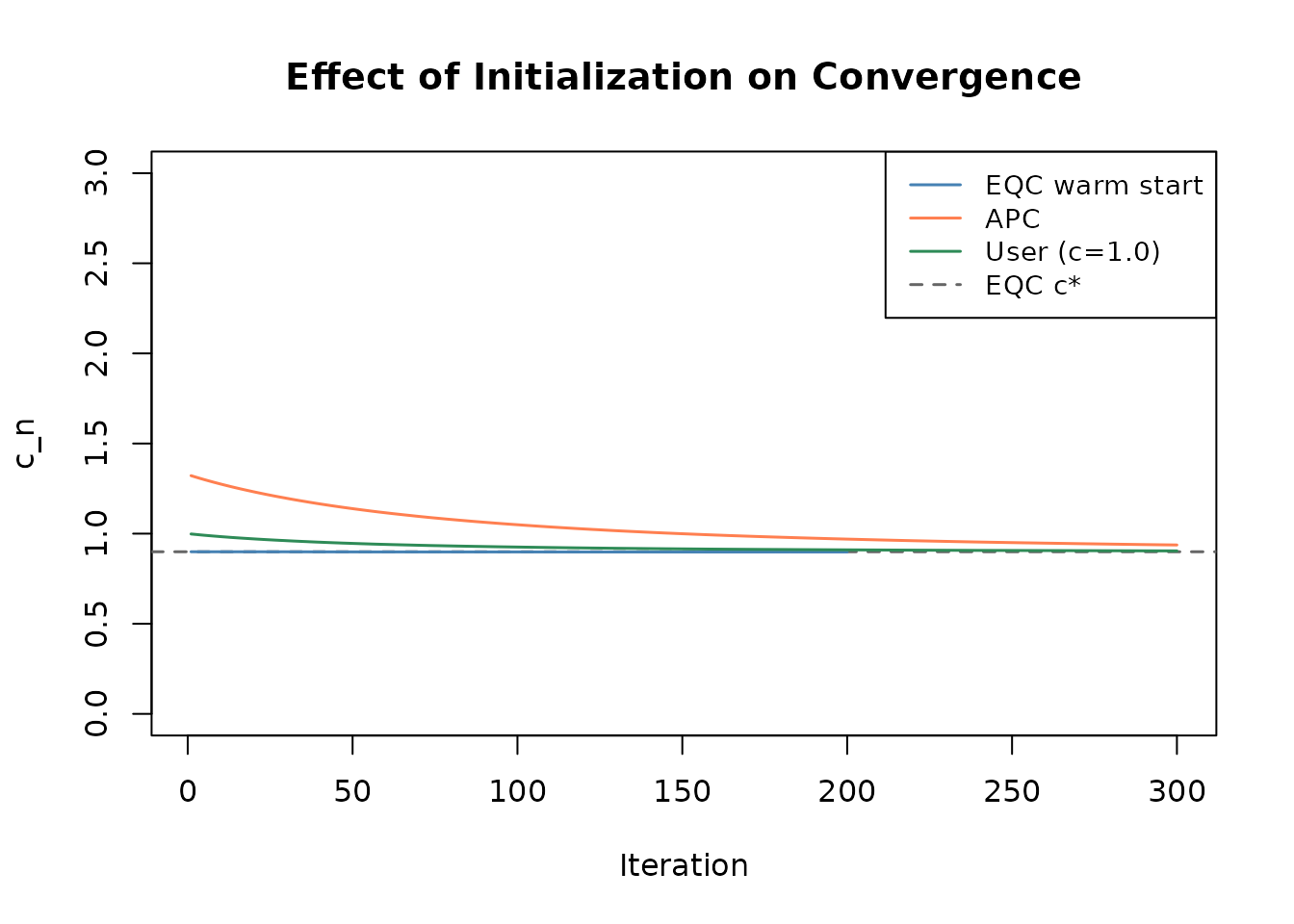

Convergence speed depends strongly on initialization quality.

Convergence Theory

Almost Sure Convergence (Theorem A.3)

Theorem (SAC Convergence; cf. Theorem A.3, Lee 2026). Suppose:

1. The step sizes satisfy Eq. (4): \sum a_n = \infty, \sum a_n^2 < \infty.
2. The reliability function \rho(c) is Lipschitz continuous on [c_L, c_U].
3. g(c) = \rho(c) - \rho^* has one isolated root c^* in the interior of the selected projected preflight branch.
4. The selected branch is globally stable over its projection interval: (c-c^*)g(c)>0 for every c\ne c^* in that interval, and g'(c^*)>0 locally.
5. The noise \varepsilon_n satisfies \mathbb{E}[\varepsilon_n \mid c_n] = 0 and \mathbb{E}[\varepsilon_n^2 \mid c_n] \leq \sigma^2_\varepsilon < \infty.

Then the projected SAC iterates converge almost surely:

c_n \xrightarrow{\text{a.s.}} c^* \quad \text{as } n \to \infty \qquad \text{(9)}

This is a local, branch-conditional result. It does not claim a globally unique root on the original user interval, and it does not apply after a reported branch_lost event. The configured preflight scan supplies numerical evidence for an increasing branch; it does not prove the branch-wide drift condition assumed by this theorem.

Proof sketch. The proof follows the classical Robbins-Monro theory, extended to the projected (constrained) setting by Kushner and Yin (2003, Chapter 5). The key steps are:

1. Lyapunov function: Define V(c) = (c - c^*)^2. Compute the conditional expectation of V(c_{n+1}) given c_n: \begin{aligned} \mathbb{E}[V(c_{n+1}) \mid c_n] &= V(c_n) - 2a_n(c_n - c^*) g(c_n) + a_n^2 \mathbb{E}[(\hat{\rho}_n - \rho^*)^2 \mid c_n] \end{aligned}

2. Drift condition: Since g(c)(c - c^*) > 0 for c \neq c^* (the reliability function is increasing, so g has the same sign as c - c^*), the drift term -2a_n(c_n - c^*)g(c_n) < 0 provides contraction toward c^*.

3. Noise control: The accumulated noise \sum a_n^2 \sigma^2_\varepsilon < \infty (by the step size conditions), so the noise does not prevent convergence.

4. Almost sure convergence: By the Robbins-Siegmund theorem (a supermartingale convergence result), V(c_n) \to V^* a.s. for some random variable V^*. The drift condition then forces V^* = 0, giving c_n \to c^* a.s.

Asymptotic Normality of Polyak-Ruppert Average

Theorem (Polyak-Ruppert CLT). Under the conditions of Theorem A.3 and additional smoothness assumptions, the Polyak-Ruppert average satisfies:

\sqrt{N - B}\,(\bar{c}_N - c^*) \xrightarrow{d} N\!\left(0,\, \frac{\sigma^2_\varepsilon}{g'(c^*)^2}\right) \qquad \text{(10)}

Under the additional regular stochastic-approximation conditions of Polyak–Juditsky theory, this covariance is asymptotically efficient for the local stochastic-approximation problem. It is not an unconditional Cramer–Rao claim for arbitrary IRT designs or noise processes.

Rate comparison: Under the same local conditions, \gamma=0.67 gives a typical last-iterate MSE order O(n^{-0.67}), whereas the Polyak–Ruppert average has O(n^{-1}) MSE and the asymptotic covariance shown above. This is the rate improvement; the reverse ordering reported in earlier documentation was incorrect.

Convergence Diagnostics

SAC provides automatic convergence assessment through several statistics.

# Run SAC with enough iterations
sac_diag <- sac_calibrate(
  target_rho = 0.80, n_items = 25, model = "rasch",
  reliability_metric = "info", resample_items = FALSE,
  c_init = eqc_for_init, n_iter = 300L, M_per_iter = 1000L,
  seed = 42, verbose = FALSE,
  preflight_controls = list(M = 500L),
  evaluation_controls = list(n_forms = 3L, M = 1000L)
)

conv <- sac_diag$convergence
cat("Convergence diagnostics:\n")
#> Convergence diagnostics:
cat(sprintf("  Converged:          %s\n", conv$converged))
#>   Converged:          TRUE
cat(sprintf("  Status:             %s\n", sac_diag$calibration_status))
#>   Status:             ok
cat(sprintf("  Status flags:       %s\n", conv$status_flags))
#>   Status flags:       ok
cat(sprintf("  Mean (first half):  %.4f\n", conv$mean_first_half))
#>   Mean (first half):  0.8981
cat(sprintf("  Mean (second half): %.4f\n", conv$mean_second_half))
#>   Mean (second half): 0.8981
cat(sprintf("  SD (post-burn-in):  %.4f\n", conv$sd_post_burn))
#>   SD (post-burn-in):  0.0001
cat(sprintf("  Hit lower bound:    %s\n", conv$hit_lower_bound))
#>   Hit lower bound:    FALSE
cat(sprintf("  Hit upper bound:    %s\n", conv$hit_upper_bound))
#>   Hit upper bound:    FALSE

Convergence criterion: The split-mean trajectory diagnostic is:

\frac{|\bar{c}_{\text{first half}} - \bar{c}_{\text{second half}}|} {\max(|c^*|, \epsilon)} < 0.05

This mean-split diagnostic detects systematic drift, which would indicate that the iterates have not yet settled around the solution. The threshold is relative to the calibrated scale because the diagnostic is measured on the c scale; \epsilon is machine precision.

The public convergence$converged flag requires all of the following:

1. enough post-burn-in iterates and the split-mean diagnostic below 5%;
2. independent achieved reliability within 0.05 of the target; and
3. no branch_lost condition (including repeated branch-bound hits, an out-of-branch final average, or a nonpositive final branch slope).

Thus the split-mean statistic alone is not the convergence decision.

Post-burn-in SD: Should be small relative to c^*. Values above 0.1 suggest more iterations or better initialization.

iteration_trace is the authoritative update ledger. Each row pairs the pre-update c_evaluated with rho_update, then records c_raw, c_updated, the reliability recomputed at that updated scale (rho_updated), and any projection. The top-level trajectory and rho_trajectory are the aligned post-update scale/reliability sequence; evaluation_trajectory (also exposed as rho_scale_trajectory) and rho_update_trajectory preserve the aligned pre-update pair. This removes the one-step pairing ambiguity present in earlier schemas.

Comparative Analysis: EQC vs SAC

When They Agree

When both algorithms use the same reliability metric and a verifiably comparable design, and the SAC run has converged, their scales can be compared. compare_eqc_sac() checks the estimand signature, model, item count, item scope, fixed bank or normalized generator specification, scale convention, and calibration status. If comparability cannot be established, it retains the side-by-side numbers but returns agreement = NA and explanatory comparability_reasons; a percentage threshold is not evidence across different estimands.

# Both targeting rho* = 0.80 with info metric
eqc_comp <- eqc_calibrate(
  target_rho = 0.80, n_items = 25, model = "rasch",
  item_source = "parametric", reliability_metric = "info",
  M = 5000L, seed = 42, verbose = FALSE
)

sac_comp <- sac_calibrate(
  target_rho = 0.80, n_items = 25, model = "rasch",
  reliability_metric = "info", resample_items = FALSE,
  c_init = eqc_comp, n_iter = 300L, M_per_iter = 1000L,
  seed = 42, verbose = FALSE,
  preflight_controls = list(M = 500L),
  evaluation_controls = list(n_forms = 3L, M = 1000L)
)

comparison <- compare_eqc_sac(eqc_comp, sac_comp, verbose = FALSE)
cat(sprintf("EQC c*:   %.4f\n", comparison$c_eqc))
#> EQC c*:   0.8995
cat(sprintf("SAC c*:   %.4f\n", comparison$c_sac))
#> SAC c*:   0.8981
cat(sprintf("Diff:     %.4f (%.2f%%)\n", comparison$diff_abs, comparison$diff_pct))
#> Diff:     0.0014 (0.15%)
cat(sprintf("Agree:    %s\n", comparison$agreement))
#> Agree:    TRUE

Sources of Disagreement

When EQC and SAC disagree by more than 5%, investigate the following:

1. Different reliability metrics: For EQC/SAC agreement checks, ensure SAC uses reliability_metric = "info". Direct SAC "msem" targeting is a different estimand, so disagreement with EQC-info is expected.

2. SAC non-convergence: Check sac_result$convergence$converged. If FALSE, increase n_iter or use EQC warm start.

3. Small M in EQC: Low quadrature size introduces Monte Carlo error. Increase M in EQC.

4. Different item scope/design: Fixed-form EQC and a resampled-form SAC target different item measures. Inspect comparable and comparability_reasons rather than interpreting their raw percentage gap.

5. Different root branch: Confirm the selected root direction and policy. A high-scale decreasing root is not interchangeable with the default lowest increasing root.

6. Extreme target: Very high (> 0.95) or very low (< 0.50) targets have flatter reliability curves, making both algorithms less precise.

What to Do When They Disagree

# Strategy 1: Increase SAC iterations
sac_longer <- sac_calibrate(
  ..., n_iter = 500L, seed = 42
)

# Strategy 2: Increase EQC quadrature
eqc_precise <- eqc_calibrate(
  ..., M = 50000L, seed = 42
)

# Strategy 3: Verify same metric
stopifnot(eqc_result$metric == sac_result$metric)

# Strategy 4: Run multiple SAC replications
sac_reps <- replicate(5, {
  sac_calibrate(
    ..., seed = sample.int(10000, 1), verbose = FALSE
  )$c_star
})
cat(sprintf("SAC c* across 5 reps: mean = %.4f, sd = %.4f\n",
            mean(sac_reps), sd(sac_reps)))

Diagnostic Examples

Trajectory Analysis

The plot() method provides visual diagnostics for SAC convergence.

# Run SAC from APC start for a more interesting trajectory
sac_traj <- sac_calibrate(
  target_rho = 0.80, n_items = 25, model = "rasch",
  item_source = "parametric", reliability_metric = "info",
  c_init = NULL,  # APC start
  n_iter = 300L, M_per_iter = 1000L,
  seed = 42, verbose = FALSE
)

plot(sac_traj, type = "c")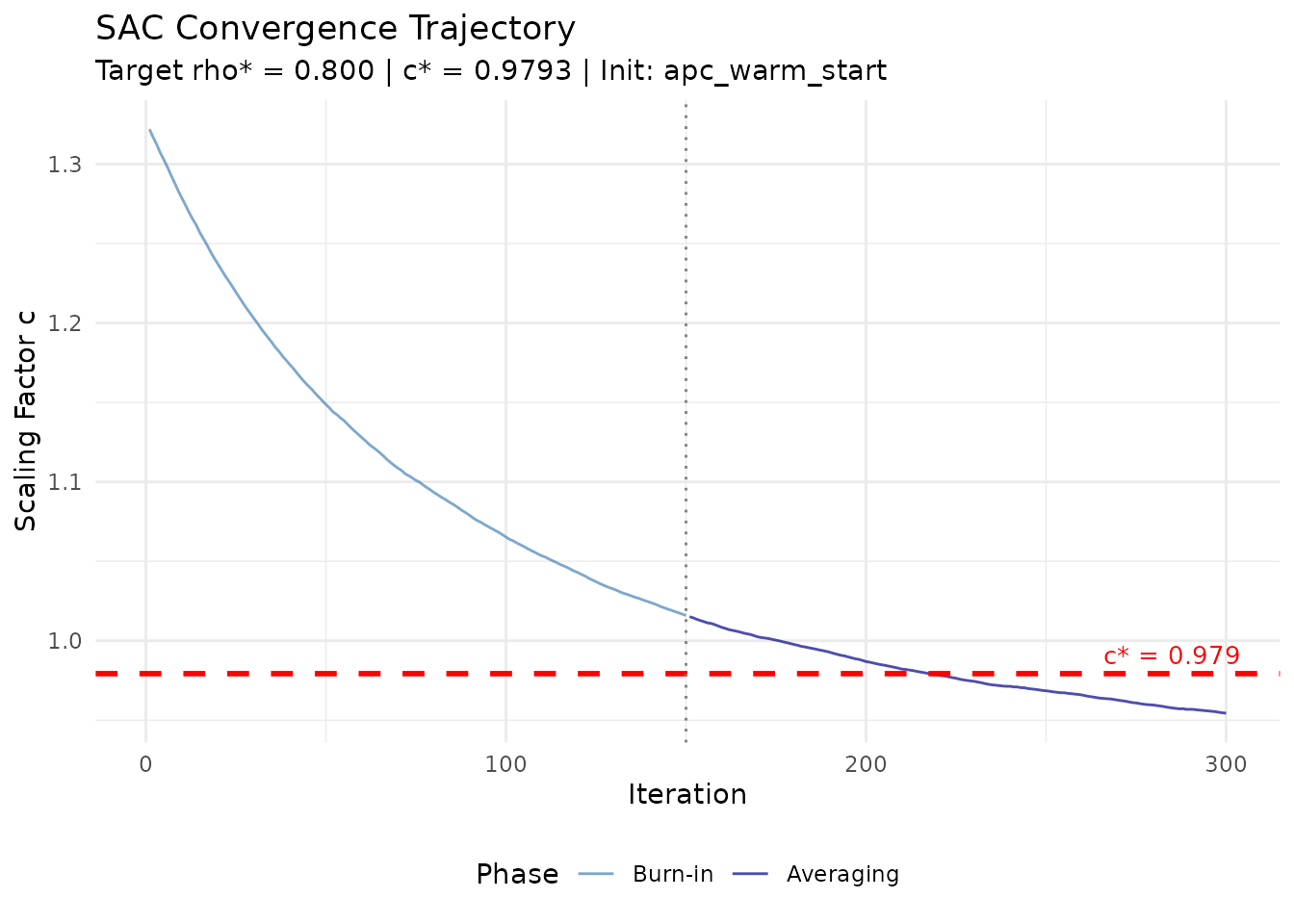

SAC convergence trajectory showing the scaling factor iterations.

plot(sac_traj, type = "rho")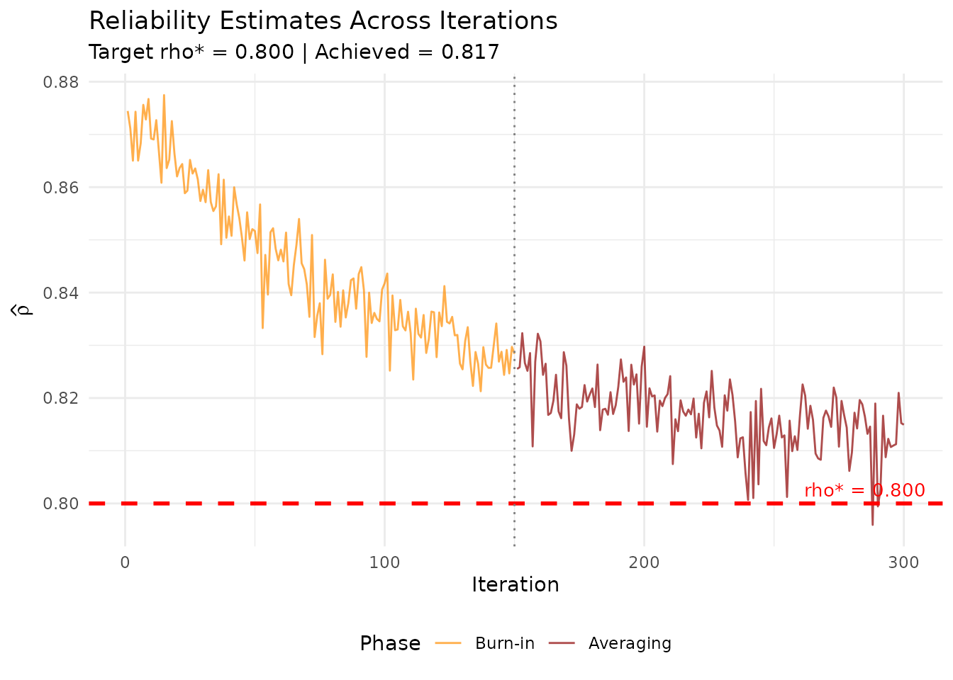

SAC reliability trajectory showing convergence to the target.

Replication Variability

SAC is inherently stochastic. Running multiple replications reveals the variability of the estimate.

n_reps <- 8
sac_reps <- numeric(n_reps)

for (r in seq_len(n_reps)) {
  sac_r <- sac_calibrate(
    target_rho = 0.80, n_items = 25, model = "rasch",
    reliability_metric = "info", resample_items = FALSE,
    c_init = eqc_for_init,
    n_iter = 200L, M_per_iter = 1000L,
    seed = r * 100, verbose = FALSE,
    preflight_controls = list(M = 500L),
    evaluation_controls = list(n_forms = 3L, M = 1000L)
  )
  sac_reps[r] <- sac_r$c_star
}

cat("SAC replication study (8 runs with EQC warm start):\n")
#> SAC replication study (8 runs with EQC warm start):
cat(sprintf("  Mean c*:  %.4f\n", mean(sac_reps)))
#>   Mean c*:  0.9031
cat(sprintf("  SD c*:    %.4f\n", sd(sac_reps)))
#>   SD c*:    0.0073
cat(sprintf("  Range:    [%.4f, %.4f]\n", min(sac_reps), max(sac_reps)))
#>   Range:    [0.8920, 0.9119]
cat(sprintf("  EQC c*:   %.4f\n", eqc_for_init$c_star))
#>   EQC c*:   0.8995
cat(sprintf("  |Mean - EQC|: %.4f\n", abs(mean(sac_reps) - eqc_for_init$c_star)))
#>   |Mean - EQC|: 0.0036

Comparison Across Different Conditions

# Test across different target reliabilities
targets <- c(0.60, 0.70, 0.80, 0.90)
cat("EQC vs SAC across target reliabilities (25 Rasch items):\n")
#> EQC vs SAC across target reliabilities (25 Rasch items):
cat(sprintf("  %-8s %-10s %-10s %-10s %-8s\n",
            "Target", "EQC c*", "SAC c*", "|Diff|", "Agree"))
#>   Target   EQC c*     SAC c*     |Diff|     Agree

for (rho_t in targets) {
  eqc_t <- eqc_calibrate(
    target_rho = rho_t, n_items = 25, model = "rasch",
    item_source = "parametric", reliability_metric = "info",
    M = 5000L, seed = 42, verbose = FALSE
  )
  sac_t <- sac_calibrate(
    target_rho = rho_t, n_items = 25, model = "rasch",
    reliability_metric = "info", resample_items = FALSE,
    c_init = eqc_t, n_iter = 200L, M_per_iter = 1000L,
    seed = 42, verbose = FALSE,
    preflight_controls = list(M = 500L),
    evaluation_controls = list(n_forms = 3L, M = 1000L)
  )
  diff_abs <- abs(eqc_t$c_star - sac_t$c_star)
  diff_pct <- 100 * diff_abs / eqc_t$c_star
  agree <- diff_pct < 5
  cat(sprintf("  %-8.2f %-10.4f %-10.4f %-10.4f %-8s\n",
              rho_t, eqc_t$c_star, sac_t$c_star, diff_abs,
              ifelse(agree, "YES", "NO")))
}
#>   0.60     0.5118     0.5111     0.0008     YES     
#>   0.70     0.6548     0.6538     0.0010     YES     
#>   0.80     0.8995     0.8982     0.0013     YES     
#>   0.90     1.5328     1.5318     0.0011     YES

Effect of M_per_iter

The per-iteration Monte Carlo sample size controls the noise level in each SAC step.

m_values <- c(200, 500, 1000, 2000)
cat("SAC sensitivity to M_per_iter (target = 0.80, 300 iter):\n")
#> SAC sensitivity to M_per_iter (target = 0.80, 300 iter):
cat(sprintf("  %-12s %-10s %-12s %-10s\n",
            "M_per_iter", "c*", "Post-burn SD", "Converged"))
#>   M_per_iter   c*         Post-burn SD Converged

for (m_val in m_values) {
  sac_m <- sac_calibrate(
    target_rho = 0.80, n_items = 25, model = "rasch",
    reliability_metric = "info", resample_items = FALSE,
    c_init = eqc_for_init, n_iter = 300L,
    M_per_iter = as.integer(m_val),
    seed = 42, verbose = FALSE,
    preflight_controls = list(M = 500L),
    evaluation_controls = list(n_forms = 3L, M = 1000L)
  )
  cat(sprintf("  %-12d %-10.4f %-12.4f %-10s\n",
              m_val, sac_m$c_star,
              sac_m$convergence$sd_post_burn,
              sac_m$convergence$converged))
}
#>   200          0.8982     0.0004       TRUE      
#>   500          0.8981     0.0002       TRUE      
#>   1000         0.8981     0.0001       TRUE      
#>   2000         0.8978     0.0001       TRUE

Independent achieved-reliability evaluation

Calibration and final evaluation use separate deterministic RNG streams. For a fixed form, independent theta blocks quantify integration variability and the concatenated evaluation nodes define achieved_rho. For an item-superpopulation target, each evaluation block has an independently drawn form and achieved_rho is the arithmetic mean of the form reliabilities; achieved_se and achieved_distribution summarize their dispersion. representative_achieved_rho and the stored representative item bank remain available for inspection, but they are not substitutes for the canonical superpopulation mean. Likewise, predict(object) returns the stored aggregate, whereas prediction at explicit new scales is labeled with its prediction scope.

The result also records preflight, branch, iteration_trace, calibration_design, evaluation_design, and rng_provenance. These fields should accompany a reproducibility report; c_star alone does not identify the estimand or branch.

Deprecated Alias

The function was previously named spc_calibrate(). For backward compatibility, spc_calibrate() still works but is deprecated and will emit a warning. Use sac_calibrate() in all new code.

Similarly, compare_eqc_spc() is deprecated in favor of compare_eqc_sac().

Summary

SAC is a theoretically grounded validation companion to EQC:

Aspect	Summary
Method	Robbins-Monro stochastic approximation
Convergence	Almost sure (Theorem A.3)
Optimal rate	O(n^{-1/2}) via Polyak-Ruppert averaging
Key advantage	Direct MSEM targeting and independent validation of EQC
Key disadvantage	Requires tuning (step size, iterations, burn-in)
Default metric	MSEM-based ("msem" / "bar"); use "info" for EQC validation
Item target	Fixed form or mean of form reliabilities, selected explicitly
Best practice	Inspect preflight/branch and independent achieved distribution; use a comparable EQC warm start only for fixed-form info calibration
Convergence check	sac_result$convergence$converged

References

Lee, J.-H. (2026). Reliability-Targeted Simulation of Item Response Data: Solving the Inverse Design Problem. arXiv:2512.16012v2. https://doi.org/10.48550/arXiv.2512.16012

Robbins, H., & Monro, S. (1951). A stochastic approximation method. The Annals of Mathematical Statistics, 22(3), 400–407.

Polyak, B. T., & Juditsky, A. B. (1992). Acceleration of stochastic approximation by averaging. SIAM Journal on Control and Optimization, 30(4), 838–855.

Kushner, H. J., & Yin, G. G. (2003). Stochastic Approximation and Recursive Algorithms and Applications (2nd ed.). Springer.

Spall, J. C. (2003). Introduction to Stochastic Search and Optimization. Wiley.