
Quick Start: Your First Calibration in 5 Minutes
JoonHo Lee (jlee296@ua.edu)
2026-08-22
Source:vignettes/quick-start.Rmd
quick-start.Rmd1. Overview
This vignette walks you through a complete IRTsimrel workflow in about five minutes. By the end you will know how to:
- Calibrate item parameters to hit a target marginal reliability.
- Check feasibility and visualize the reliability curve.
- Generate a simulated binary response dataset.
- Extract and inspect calibrated parameters using S3 methods.
- Extend the same workflow to a 3PL test with lower asymptotes.
Estimated time: 5 minutes.
Prerequisites: Only the IRTsimrel package is needed. The executable chunks in the walkthrough run on any system with the current IRTsimrel version installed; the final full-workflow block is shown as a copyable template.
2. Calibrate
The core function is eqc_calibrate(). Give it a target
reliability, the number of items, and a measurement model, and it
returns a calibrated scaling factor c^*
that makes the selected empirical reliability objective match your
target. Population accuracy remains a Monte Carlo approximation and is
best assessed on independent draws.
result <- eqc_calibrate(
  target_rho = 0.80,
  n_items    = 20,
  model      = "rasch",
  reliability_metric = "info",
  seed       = 42,
  M          = 5000L
)
Print the result to see the key quantities:
result
#>
#> =======================================================
#>   Empirical Quadrature Calibration (EQC) Results
#> =======================================================
#>
#> Calibration Summary:
#>   Model                        : RASCH
#>   Target reliability (rho*)    : 0.8000
#>   Achieved reliability         : 0.8000
#>   Absolute error               : 1.08e-07
#>   Scaling factor (c*)          : 1.0183
#>
#> Design Parameters:
#>   Number of items (I)          : 20
#>   Quadrature points (M)        : 5000
#>   Reliability metric           : Average-information (tilde)
#>   Latent variance              : 1.0099
#>
#> Convergence:
#>   Root status                  : uniroot_success
#>   Calibration status           : ok
#>   Roots detected               : 1
#>   Search bracket               : [0.300, 3.000]
#>   Bracket reliabilities        : [0.3054, 0.9471]
#>
#> Parameter Summaries:
#>   theta:        mean = -0.014, sd = 1.005
#>   beta:         mean = -0.000, sd = 0.758, range = [-2.15, 1.12]
#>   lambda_base:  mean = 1.000, sd = 0.000
#>   lambda_scaled: mean = 1.018, sd = 0.000
There are two numbers to focus on in the output:
c*(scaling factor): All baseline discriminations are multiplied by this value. In a Rasch model the baseline discriminations are all 1, so the calibrated discriminations equal c^* directly. A larger c^* means the test needs more discriminating items to reach the target.achieved_rho: The empirical reliability at the calibrated c^*, computed over the Monte Carlo quadrature sample. This should be very close to the target of 0.80 — typically the absolute error is less than 10^{-4}.
The model argument accepts "rasch" (all
discriminations equal), "2pl" (varying discriminations), or
"3pl" (varying discriminations plus item lower asymptotes).
For this first pass we use the Rasch model so the familiar v0.2 workflow
is unchanged. A compact, executable 3PL version appears in Section
7.
3. Check Feasibility
Before committing to a particular simulation design, it is good practice to verify that your target reliability is actually achievable. Not all combinations of test length, model, and latent distribution can produce every reliability level.
check_feasibility() reports the range of achievable
reliabilities for a given configuration:
feas <- check_feasibility(
  n_items   = 20,
  model     = "rasch",
  target_rho = 0.80,
  seed      = 42,
  M         = 5000L,
  verbose   = FALSE
)
feas
#>
#> =======================================================
#>   Feasibility Check: Achievable Reliability Range
#> =======================================================
#>
#>   Number of items  : 20
#>   Model            : RASCH
#>   Latent shape     : normal
#>   Latent variance  : 1.0099
#>   c range          : [0.10, 10.00]
#>   Monte Carlo M    : 5000
#>
#> Achievable Reliability Ranges:
#>   rho_tilde (info) : [0.0479, 0.9850]
#>   rho_bar   (msem) : [0.0000, 0.8818]
#>
#> Target rho*        : 0.8000
#>   info status      : feasible
#>   msem status      : feasible
#>
#> Note: rho_tilde >= rho_bar on the same information grid (Jensen's inequality).
#>   rho_tilde range screens EQC targets; root policy must still admit a root.
#>   rho_bar range screens SAC targets; stable interior-branch preflight is also required.
The output shows two finite-sample ranges, one for each metric. Range
membership is a screening condition, not by itself a calibration
guarantee: inspect the canonical target status, detected roots,
admissible-root counts, and topology resolution. EQC additionally needs
a root admitted by its root_policy. SAC performs its own
split-bank preflight and requires a stable interior increasing crossing.
It also rejects population-MSEM targeting for the built-in
heavy_tail distribution because that functional can be
non-integrable even when a finite grid returns a number.
You can also visualize how reliability varies continuously with the
scaling factor by using rho_curve(). This plot shows both
the average-information metric (\tilde{\rho}, blue) and the MSEM-based metric
(\bar{w}, red):
curve_data <- rho_curve(
  n_items = 20,
  model   = "rasch",
  metric  = "both",
  M       = 5000L,
  seed    = 42,
  plot    = TRUE
)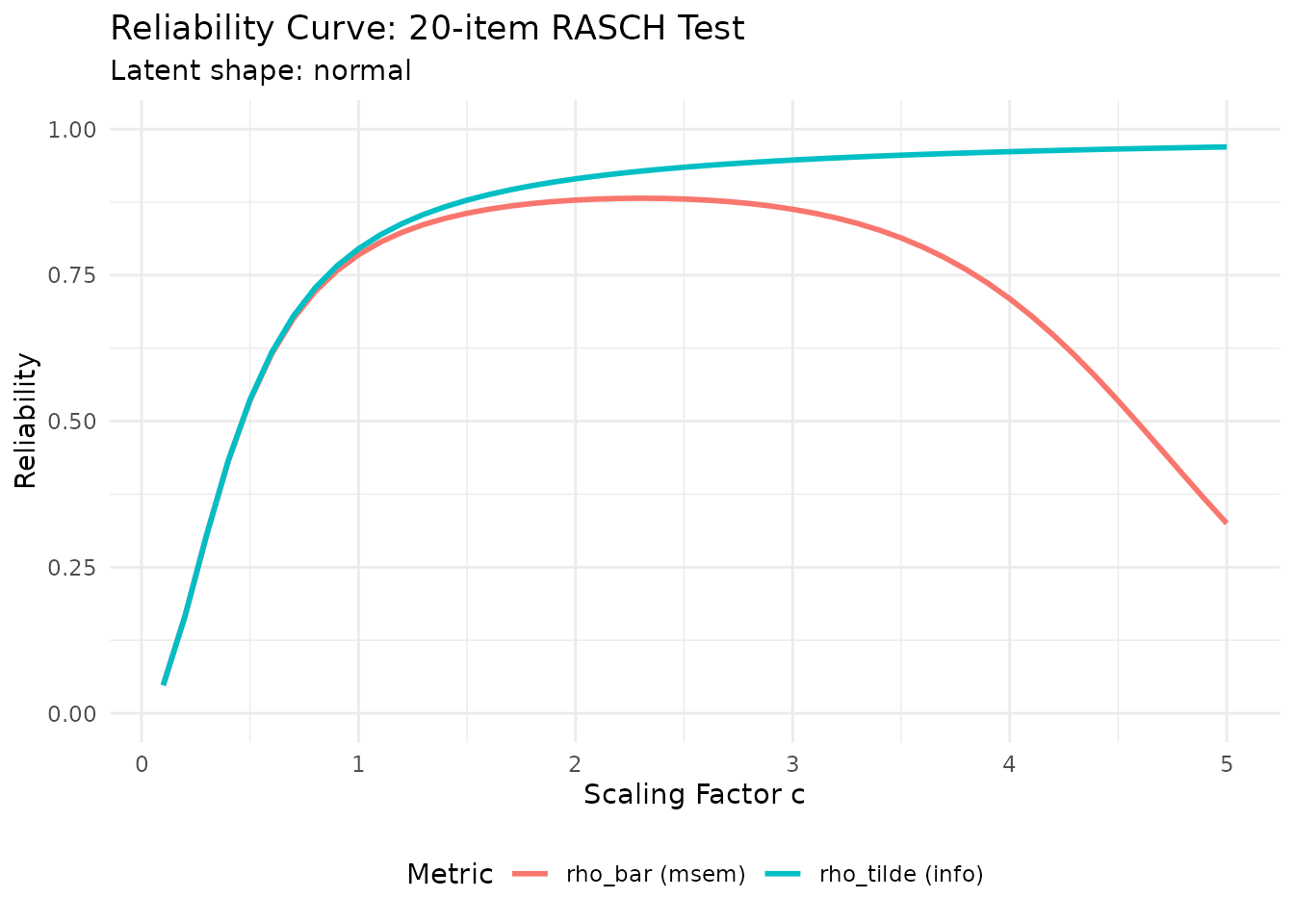
Reliability curve for a 20-item Rasch test. On the same quadrature grid, the average-information metric (blue) lies at or above the MSEM-based metric (red) due to Jensen’s inequality.
The two curves are close together for this configuration. The gap widens for shorter tests or non-normal latent distributions.
4. Generate Data
Once you have a calibration result,
simulate_response_data() generates a binary response matrix
using the calibrated item parameters. The function draws fresh latent
abilities from the specified distribution and produces responses
according to the stored Rasch, 2PL, or 3PL model with the calibrated
discriminations:
sim <- simulate_response_data(
  result    = result,
  n_persons = 500,
  seed      = 123
)
The result is a list with five components:
-
response_matrix: an N \times I matrix of binary (0/1) responses -
theta: the true latent abilities for each person -
beta: the item difficulties -
lambda: the scaled item discriminations -
guessing: item lower asymptotes (zero for Rasch/2PL) -
provenance: calibration and simulation metadata, including metric, status, item source, and seed
# Dimensions: 500 persons x 20 items
dim(sim$response_matrix)
#> [1] 500  20
sim$provenance[c("metric", "calibration_status", "status_flags", "item_source")]
#> $metric
#> [1] "info"
#>
#> $calibration_status
#> [1] "uniroot_success"
#>
#> $status_flags
#> [1] "uniroot_success"
#>
#> $item_source
#> [1] "parametric"
# First 6 persons, first 8 items
sim$response_matrix[1:6, 1:8]
#>      item1 item2 item3 item4 item5 item6 item7 item8
#> [1,]     0     1     0     1     0     0     0     0
#> [2,]     0     1     0     1     1     0     1     0
#> [3,]     1     1     1     1     1     1     1     1
#> [4,]     1     0     0     1     0     1     1     1
#> [5,]     1     0     0     0     1     1     0     0
#> [6,]     1     1     1     1     1     1     1     1
You can verify that the item parameters match what you expect:
# All scaled discriminations should equal c*
summary(sim$lambda)
#>    Min. 1st Qu.  Median    Mean 3rd Qu.    Max.
#>   1.018   1.018   1.018   1.018   1.018   1.018

# Difficulty distribution
summary(sim$beta)
#>     Min.  1st Qu.   Median     Mean  3rd Qu.     Max.
#> -2.14978 -0.33975  0.04838  0.00000  0.37403  1.12028
A quick diagnostic: plot the proportion of correct responses per item. Items with extreme difficulties should have very high or very low proportions:
p_correct <- colMeans(sim$response_matrix)
item_order <- order(sim$beta)

barplot(
  p_correct[item_order],
  names.arg = item_order,
  col  = "steelblue",
  xlab = "Item (ordered by difficulty)",
  ylab = "Proportion Correct",
  main = "Proportion Correct per Item",
  ylim = c(0, 1),
  las  = 2,
  cex.names = 0.7
)
abline(h = 0.5, lty = 2, col = "gray50")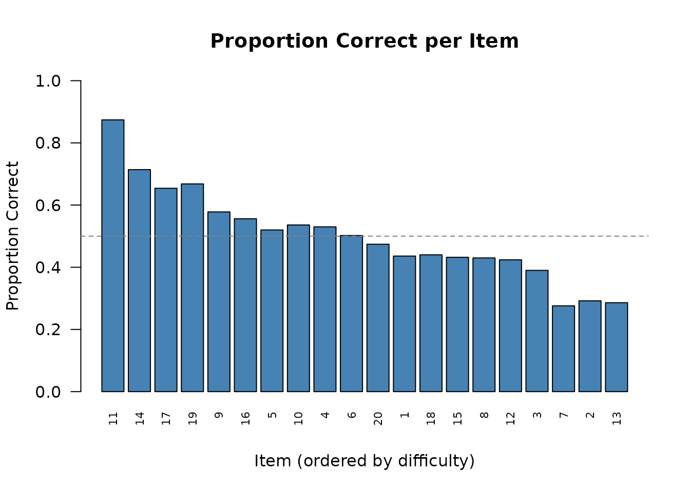
Proportion correct per item, ordered by difficulty. Items near the center of the difficulty distribution have proportions near 0.50, while extreme items show floor or ceiling effects.
5. Extract and Inspect
IRTsimrel result objects support standard S3 generics, so you can
interact with them the same way you would with lm or
glm objects.
5.1 Summary
summary() returns a compact overview of the
calibration:
summary(result)
#> Summary: Empirical Quadrature Calibration (EQC)
#> ================================================
#>   Model            : RASCH
#>   Metric           : Average-information (tilde)
#>   Number of items  : 20
#>   Quadrature (M)   : 5000
#>   Latent variance  : 1.0099
#>
#> Calibration Results:
#>   Target rho*      : 0.8000
#>   Achieved rho     : 0.8000
#>   Absolute error   : 1.08e-07
#>   Scaling factor c*: 1.0183
#>   Root status      : uniroot_success
#>   Calibration      : ok
#>   Roots detected   : 1
5.2 Extract Coefficients
coef() returns a tidy data frame of calibrated item
parameters — one row per item:
item_pars <- coef(result)
head(item_pars)
#>   item_id         beta lambda_base lambda_scaled   c_star
#> 1       1  0.217684472           1      1.018302 1.018302
#> 2       2  1.116752062           1      1.018302 1.018302
#> 3       3  0.456497288           1      1.018302 1.018302
#> 4       4  0.006913473           1      1.018302 1.018302
#> 5       5 -0.179849098           1      1.018302 1.018302
#> 6       6  0.027652529           1      1.018302 1.018302
For a Rasch model, lambda_base is always 1 and
lambda_scaled equals c^*
for every item. For 2PL and 3PL models, lambda_base varies
across items and lambda_scaled is
lambda_base * c*. A 3PL coefficient table also contains
guessing; calibration does not multiply that column by
c^*.
5.3 Predict Reliability at New Scaling Factors
predict() evaluates the reliability function at new
scaling factor values. With no arguments, it returns the achieved
reliability at the calibrated c^*:
# Achieved reliability at c*
predict(result)
#> [1] 0.8000001
With newdata, it computes reliability at each specified
value of c:
# Reliability at several scaling factors
predict(result, newdata = c(0.5, 1.0, 1.5, 2.0))
#>     c=0.5     c=1.0     c=1.5     c=2.0
#> 0.5369213 0.7952739 0.8784820 0.9150086
This is useful for understanding how sensitive reliability is to the discrimination level. For instance, at c = 0.5 the test is substantially less reliable, while at c = 2.0 it is more reliable than needed.
6. Validate (Optional)
For added confidence in your calibration, you can run SAC (Stochastic
Approximation Calibration) as an independent check. SAC uses a
completely different algorithm (Robbins-Monro stochastic approximation).
When validating an EQC result, set
reliability_metric = "info" so both algorithms solve the
same calibration problem; agreement is then strong evidence that both
found the correct c^*.
Passing the EQC result as c_init provides a warm start
that makes SAC converge in very few iterations:
sac_result <- sac_calibrate(
  target_rho = 0.80,
  n_items    = 20,
  model      = "rasch",
  reliability_metric = "info",
  c_init     = result,
  resample_items = FALSE,
  n_iter     = 100L,
  M_per_iter = 500L,
  seed       = 42
)
Compare the two algorithms side by side:
comp <- compare_eqc_sac(result, sac_result)
#>
#> =======================================================
#>   EQC vs SAC Comparison
#> =======================================================
#>
#>   Target reliability  : 0.8000
#>   EQC c*              : 1.018302
#>   SAC c*              : 1.017653
#>   Absolute difference : 0.000648
#>   Percent difference  : 0.06%
#>   EQC achieved rho    : 0.8000
#>   SAC achieved rho    : 0.8004
#>   Comparable           : YES
#>   Agreement (< 5%)    : YES
#>   Agreement status     : evaluated
#>   EQC status          : uniroot_success
#>   SAC status          : ok
#>   SAC status flags    : ok
#>
The comparison reports the absolute and percent difference between
the two c^* values and applies its 5%
diagnostic agreement threshold. Interpret that flag together with
comparable, calibration status, and the independent holdout
reliability rather than as a universal precision guarantee.
You can also visualize the SAC convergence trajectory to verify that the iterations stabilized near the EQC warm start:
plot(sac_result, type = "both")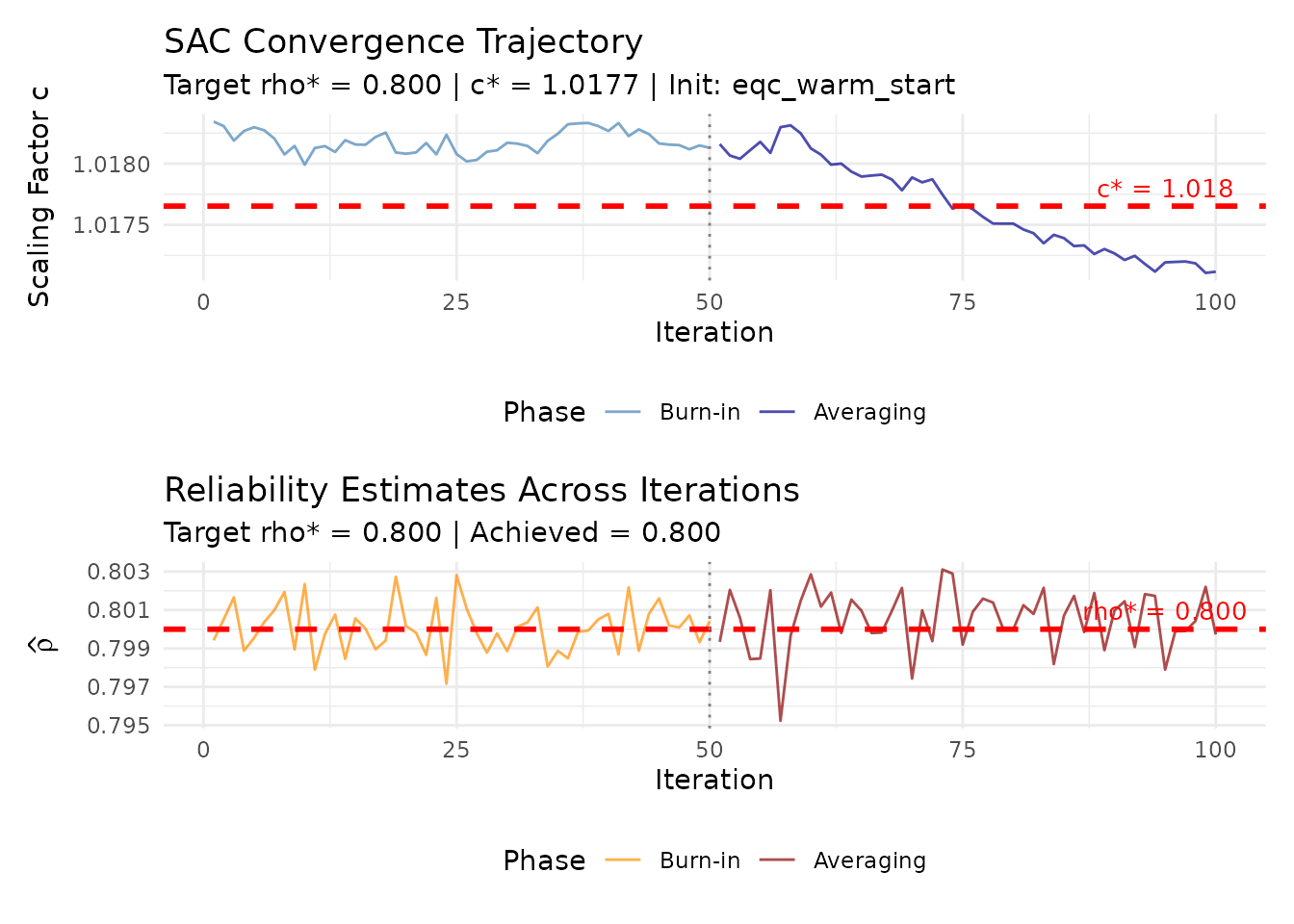
SAC convergence trajectory. The top panel shows the scaling factor c across iterations, and the bottom panel shows the per-iteration reliability estimates. The warm start from EQC ensures rapid convergence.
The top panel shows the scaling factor trajectory, which should stabilize quickly when initialized from EQC. The bottom panel shows the noisy per-iteration reliability estimates oscillating around the target value (dashed red line). The Polyak-Ruppert average (reported as c^*) smooths out the iteration-to-iteration noise.
7. Putting It All Together
Here is the complete workflow in a single code block, from calibration to validated data generation:
library(IRTsimrel)

# Step 1: Check feasibility
feas <- check_feasibility(
  n_items = 20, model = "rasch", target_rho = 0.80,
  seed = 42, verbose = FALSE
)

# Step 2: Calibrate with EQC
eqc_res <- eqc_calibrate(
  target_rho = 0.80, n_items = 20, model = "rasch",
  reliability_metric = "info", seed = 42, M = 5000L
)

# Step 3: Validate with SAC (optional but recommended)
sac_res <- sac_calibrate(
  target_rho = 0.80, n_items = 20, model = "rasch",
  reliability_metric = "info", c_init = eqc_res,
  resample_items = FALSE, n_iter = 100L, seed = 42
)
compare_eqc_sac(eqc_res, sac_res)

# Step 4: Generate response data
sim_data <- simulate_response_data(
  result = eqc_res, n_persons = 1000, seed = 123
)

# Step 5: Use the data in your analysis
dim(sim_data$response_matrix)  # 1000 x 20
8. The Same Cycle for a 3PL Test
The 3PL response probability is
P(Y_i=1\mid\theta)=g_i+(1-g_i) \operatorname{logit}^{-1}\{c\lambda_{i,0}(\theta-\beta_i)\}.
Here guessing_params generates the lower asymptotes
g_i. In contrast, scale in
sim_item_params() and the calibrated c^* are the same kind of global
discrimination multiplier: they change \lambda, not g. The names are deliberately kept separate
in the API to prevent treating a 0.20 guessing parameter as a
discrimination scale.
The following small workflow generates a fixed 3PL form, calibrates it with EQC, validates the same estimand with a fixed-form SAC run, and then generates responses. The seeds are explicit, and the vignette-sized Monte Carlo settings keep the example fast.
# Generate and freeze one item form.
items_3pl <- sim_item_params(
  n_items = 12,
  model = "3pl",
  source = "parametric",
  guessing_params = list(distribution = "fixed", value = 0.20),
  seed = 310
)

fixed_3pl <- list(custom_params = list(
  beta = items_3pl$data$beta,
  lambda = items_3pl$data$lambda_unscaled,
  guessing = items_3pl$data$guessing
))

eqc_3pl <- eqc_calibrate(
  target_rho = 0.70,
  n_items = 12,
  model = "3pl",
  item_source = "custom",
  item_params = fixed_3pl,
  reliability_metric = "info",
  M = 2000L,
  seed = 310
)

# Omitted item_source/item_params tell SAC to reuse the EQC form exactly.
sac_3pl <- sac_calibrate(
  target_rho = 0.70,
  n_items = 12,
  model = "3pl",
  reliability_metric = "info",
  c_init = eqc_3pl,
  resample_items = FALSE,
  n_iter = 60L,
  M_per_iter = 250L,
  M_pre = 1000L,
  evaluation_controls = list(n_forms = 3L, M = 500L),
  seed = 310
)

responses_3pl <- simulate_response_data(
  result = eqc_3pl,
  n_persons = 200,
  seed = 311
)

validation_3pl <- compare_eqc_sac(eqc_3pl, sac_3pl)
#>
#> =======================================================
#>   EQC vs SAC Comparison
#> =======================================================
#>
#>   Target reliability  : 0.7000
#>   EQC c*              : 1.183123
#>   SAC c*              : 1.171030
#>   Absolute difference : 0.012093
#>   Percent difference  : 1.02%
#>   EQC achieved rho    : 0.7000
#>   SAC achieved rho    : 0.7045
#>   Comparable           : YES
#>   Agreement (< 5%)    : YES
#>   Agreement status     : evaluated
#>   EQC status          : uniroot_success
#>   SAC status          : ok
#>   SAC status flags    : ok
#>
stopifnot(
  validation_3pl$comparable,
  identical(dim(responses_3pl$response_matrix), c(200L, 12L)),
  all(responses_3pl$guessing == 0.20)
)
head(coef(eqc_3pl))
#>   item_id       beta lambda_base lambda_scaled   c_star guessing
#> 1       1 -1.1690253   1.0633685      1.258095 1.183123      0.2
#> 2       2  0.9058676   0.9813886      1.161103 1.183123      0.2
#> 3       3  0.2164509   1.5745857      1.862928 1.183123      0.2
#> 4       4  0.7229356   1.3660700      1.616228 1.183123      0.2
#> 5       5  1.8519541   0.8899961      1.052975 1.183123      0.2
#> 6       6 -0.7876383   1.2991184      1.537017 1.183123      0.2
EQC always targets the generated fixed form. For
SAC, resample_items = FALSE targets that same fixed form,
whereas resample_items = TRUE targets an item
superpopulation by drawing forms during calibration and
reporting the mean reliability across independent holdout forms. An EQC
object is therefore a valid SAC warm start only for the same metric and
fixed item bank; use a numeric or automatic SAC initializer for a
superpopulation run.
Setting all g_i=0 gives exact nested 2PL behavior in the response and information kernels. Existing Rasch/2PL calls need no new arguments, so this extension is backward compatible.
9. What’s Next?
You have now completed a full calibrate-generate-validate cycle. Here are some directions for deeper exploration:
vignette("applied-guide"): Comprehensive applied tutorial covering Rasch, 2PL, and 3PL models; fixed-form versus item-superpopulation targets; non-normal latent distributions; optional IRW-based item sources; and factorial simulation designs with multiple reliability levels.vignette("latent-distributions"): Explore all 12 latent distribution shapes available insim_latentG()and learn when to use each one for different research scenarios.vignette("item-parameters"): Parametric, IRW, hierarchical, and custom item generation methods, including correlated difficulty-discrimination parameters.vignette("theory-reliability"): Mathematical foundations of the two reliability metrics (\tilde{\rho} and \bar{w}), Jensen’s inequality, and the theoretical justification for the calibration approach.vignette("api-reference"): Full function reference with complete signatures, all arguments, return values, and runnable examples for every exported function.
References
Lee, J.-H. (2026). Reliability-Targeted Simulation of Item Response Data: Solving the Inverse Design Problem. arXiv:2512.16012v2. https://doi.org/10.48550/arXiv.2512.16012