Applied Guide: Reliability-Targeted IRT Simulation

1. Overview

Reading time: approximately 30–40 minutes.

This vignette walks through the complete workflow for generating simulated item response data with a pre-specified marginal reliability. The approach implements the framework described in Lee (2026), which treats reliability as a design parameter rather than an emergent property of the simulation.

Learning objectives. After completing this guide you will be able to:

Screen whether a desired reliability is achievable for a given test design.
Visualize the reliability curve to understand the design space.
Calibrate a discrimination scaling factor with EQC (Algorithm 1).
Optionally validate the calibration with SAC (Algorithm 2).
Generate item response data at the target reliability.
Extract, summarize, and export calibrated item parameters.
Distinguish fixed-form from item-superpopulation targets in 3PL work.

Prerequisites. Install IRTsimrel and, optionally, TAM for external Rasch/2PL validation and 3PL EAP diagnostics:

# install.packages("devtools")
devtools::install_github("joonho112/IRTsimrel")
install.packages("TAM")

In the TAM version used for the package’s v0.3 validation, a 3PL fit supports EAP scoring but not tam.wle() on the tam.mml.3pl object. Do not coerce the object class or report a 3PL TAM WLE result through an unsupported path.

Most baseline examples use seed = 42 and M = 5000L; the compact 3PL workflow uses smaller documented settings and separate seeds so the vignette remains quick and reproducible. Treat these as tutorial settings, not automatic precision recommendations for a final study.

2. The 6-Step Workflow

The reliability-targeted simulation workflow consists of six steps. The table below provides a quick summary before we walk through each step in detail.

Step	Function	Purpose
1	`check_feasibility()`	Screen whether \rho^* is achievable
2	`rho_curve()`	Visualize \rho(c) across scaling factors
3	`eqc_calibrate()`	Find c^* such that \rho(c^) \approx \rho^
4	`sac_calibrate()`	(Optional) Validate c^* via stochastic approximation
5	`simulate_response_data()`	Generate binary response matrix
6	`coef()`, `predict()`, `as.data.frame()`	Extract and use results

2.1 Step 1: Screen Feasibility with `check_feasibility()`

Before investing computation time in calibration, verify that the target reliability is achievable. check_feasibility() evaluates both reliability metrics across a range of scaling factors and reports the achievable interval.

feas <- check_feasibility(
  n_items      = 25,
  model        = "rasch",
  latent_shape = "normal",
  item_source  = "parametric",
  target_rho   = 0.85,
  c_bounds     = c(0.1, 10),
  M            = 5000L,
  seed         = 42
)
#> 
#> =======================================================
#>   Feasibility Check: Achievable Reliability Range
#> =======================================================
#> 
#>   Number of items  : 25
#>   Model            : RASCH
#>   Latent shape     : normal
#>   Latent variance  : 1.0099
#>   c range          : [0.10, 10.00]
#>   Monte Carlo M    : 5000
#> 
#> Achievable Reliability Ranges:
#>   rho_tilde (info) : [0.0591, 0.9872]
#>   rho_bar   (msem) : [0.0002, 0.9146]
#> 
#> Target rho*        : 0.8500
#>   info status      : feasible
#>   msem status      : feasible
#> 
#> Note: rho_tilde >= rho_bar on the same information grid (Jensen's inequality).
#>   rho_tilde range screens EQC targets; root policy must still admit a root.
#>   rho_bar range screens SAC targets; stable interior-branch preflight is also required.

The output reports the resolved range for both the average-information metric (\tilde{\rho}) and the MSEM-based metric (\bar{w}) in one finite Monte Carlo design. If a target falls outside that range, it is infeasible within the configured bounds and sampled design. Inspect the topology and best-achievable record before deciding whether to justify wider bounds, add items, or change the item model. A finite heavy-tail MSEM range is sensitivity evidence only, not a population feasibility certificate.

Quick check for a specific target:

target <- 0.85
in_range <- identical(feas$target_status_info_canonical, "feasible")
admissible <- feas$admissible_root_count_info > 0L
cat(sprintf("Target rho = %.2f is %s for this design.\n",
            target,
            ifelse(in_range && admissible,
                   "FEASIBLE WITH AN ADMISSIBLE ROOT",
                   "NOT YET CALIBRATION-READY")))
#> Target rho = 0.85 is FEASIBLE WITH AN ADMISSIBLE ROOT for this design.

Comparing feasibility across designs

You can compare different test lengths to find the minimum number of items needed:

test_lengths <- c(10, 15, 20, 25, 30, 40)
feas_table <- data.frame(
  n_items   = test_lengths,
  rho_min   = numeric(length(test_lengths)),
  rho_max   = numeric(length(test_lengths))
)

for (i in seq_along(test_lengths)) {
  fi <- check_feasibility(
    n_items = test_lengths[i], model = "rasch",
    item_source = "parametric", target_rho = target, M = 5000L,
    seed = 42, verbose = FALSE
  )
  feas_table$rho_min[i] <- round(fi$rho_range_info[1], 4)
  feas_table$rho_max[i] <- round(fi$rho_range_info[2], 4)
}

feas_table
#>   n_items rho_min rho_max
#> 1      10  0.0246  0.9729
#> 2      15  0.0363  0.9797
#> 3      20  0.0479  0.9850
#> 4      25  0.0591  0.9872
#> 5      30  0.0701  0.9894
#> 6      40  0.0914  0.9918

plot(NULL, xlim = range(test_lengths), ylim = c(0, 1),
     xlab = "Number of Items", ylab = expression(tilde(rho)),
     main = "Achievable Reliability Range by Test Length")
polygon(c(test_lengths, rev(test_lengths)),
        c(feas_table$rho_min, rev(feas_table$rho_max)),
        col = adjustcolor("steelblue", alpha.f = 0.3), border = NA)
lines(test_lengths, feas_table$rho_min, col = "steelblue", lwd = 2)
lines(test_lengths, feas_table$rho_max, col = "steelblue", lwd = 2)
abline(h = 0.85, lty = 2, col = "firebrick")
text(max(test_lengths), 0.86, expression(rho^"*" == 0.85),
     col = "firebrick", pos = 2, cex = 0.9)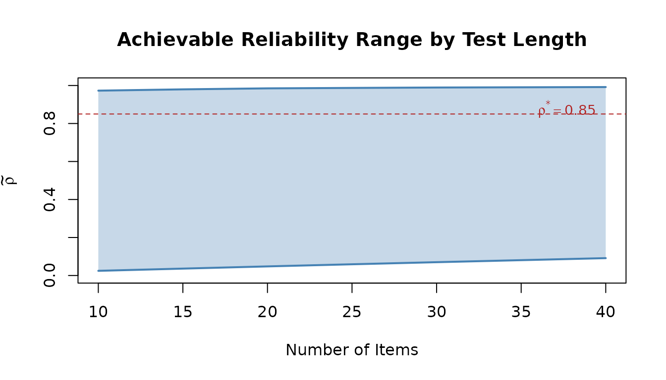

Line plot of achievable reliability ranges by test length with the target reliability shown as a horizontal reference line.

The shaded region shows the achievable reliability range as a function of test length. This type of visualization is useful for study planning: you can immediately see the minimum test length needed to reach your desired reliability.

For more on how the latent distribution affects these ranges, see vignette("latent-distributions").

2.2 Step 2: Explore the Reliability Curve with `rho_curve()`

The reliability curve \rho(c) shows how reliability changes as the global discrimination scaling factor c varies. This visualization helps you understand the shape of the design space and select sensible targets.

curve_data <- rho_curve(
  n_items      = 25,
  model        = "rasch",
  latent_shape = "normal",
  item_source  = "parametric",
  metric       = "both",
  M            = 5000L,
  seed         = 42,
  plot         = TRUE
)

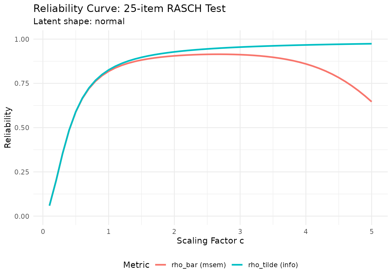
Reliability curve showing how reliability changes with the discrimination scaling factor for the selected design.

The plot shows both \tilde{\rho} (average-information) and \bar{w} (MSEM-based). Note that \tilde{\rho} \geq \bar{w} holds on the same population/grid basis by Jensen’s inequality.

Reading the curve. You can use the returned data frame to find approximate c values for any target:

head(curve_data)
#> Reliability Curve
#> =================
#>   Items: 25 | Model: RASCH | Metric: both
#>   c range: [0.10, 0.60] (6 points)
#>   rho_tilde range: [0.0591, 0.6666]
#>   rho_bar range  : [0.0591, 0.6641]
#> 
#>     c  rho_tilde    rho_bar
#> 1 0.1 0.05913372 0.05913302
#> 2 0.2 0.19889655 0.19886569
#> 3 0.3 0.35385665 0.35364731
#> 4 0.4 0.48680763 0.48614470
#> 5 0.5 0.58967106 0.58825103
#> 6 0.6 0.66655958 0.66412727

# Find approximate c for rho_tilde = 0.80
idx <- which.min(abs(curve_data$rho_tilde - 0.80))
cat(sprintf("Approximate c for rho_tilde = 0.80: %.3f\n", curve_data$c[idx]))
#> Approximate c for rho_tilde = 0.80: 0.900

2.3 Step 3: Calibrate with EQC — `eqc_calibrate()`

EQC (Empirical Quadrature Calibration) is Algorithm 1 from Lee (2026). It maps the empirical reliability topology on the requested log-scale interval, selects a branch under root_policy, and uses Brent’s method via uniroot() only to polish ordinary sign-changing crossings of \hat{\rho}_M(c^*) = \rho^*.

2.3.1 Basic calibration (Rasch)

eqc_result <- eqc_calibrate(
  target_rho        = 0.85,
  n_items           = 25,
  model             = "rasch",
  latent_shape      = "normal",
  item_source       = "parametric",
  reliability_metric = "info",
  M                 = 5000L,
  seed              = 42,
  verbose           = TRUE
)
#> Step 1: Generating quadrature samples...
#>   M (quad persons) = 5000
#>   I (items)        = 25
#>   theta: mean = -0.014, sd = 1.005, var = 1.010
#>   beta:  mean = 0.000, sd = 0.861
#>   lambda_base: mean = 1.000, sd = 0.000
#>   metric = info
#> Step 2: Running root-finding algorithm...
#>   At c = 0.300: rho = 0.3539, g = -0.4961
#>   At c = 3.000: rho = 0.9550, g = 0.1050
#>   c* = 1.119883
#>   Target rho    = 0.8500
#>   Achieved rho  = 0.8500
#>   Root status   = uniroot_success

print(eqc_result)
#> 
#> =======================================================
#>   Empirical Quadrature Calibration (EQC) Results
#> =======================================================
#> 
#> Calibration Summary:
#>   Model                        : RASCH
#>   Target reliability (rho*)    : 0.8500
#>   Achieved reliability         : 0.8500
#>   Absolute error               : 4.21e-07
#>   Scaling factor (c*)          : 1.1199
#> 
#> Design Parameters:
#>   Number of items (I)          : 25
#>   Quadrature points (M)        : 5000
#>   Reliability metric           : Average-information (tilde)
#>   Latent variance              : 1.0099
#> 
#> Convergence:
#>   Root status                  : uniroot_success
#>   Calibration status           : ok
#>   Roots detected               : 1
#>   Search bracket               : [0.300, 3.000]
#>   Bracket reliabilities        : [0.3539, 0.9550]
#> 
#> Parameter Summaries:
#>   theta:        mean = -0.014, sd = 1.005
#>   beta:         mean = 0.000, sd = 0.861, range = [-2.17, 1.45]
#>   lambda_base:  mean = 1.000, sd = 0.000
#>   lambda_scaled: mean = 1.120, sd = 0.000

Key outputs:

c_star: the calibrated scaling factor c^*.
achieved_rho: the empirical reliability at c^*.
items_calib: the item parameter object with scaled discriminations.

2.3.2 Exploring the result

summary(eqc_result)
#> Summary: Empirical Quadrature Calibration (EQC)
#> ================================================
#>   Model            : RASCH
#>   Metric           : Average-information (tilde)
#>   Number of items  : 25
#>   Quadrature (M)   : 5000
#>   Latent variance  : 1.0099
#> 
#> Calibration Results:
#>   Target rho*      : 0.8500
#>   Achieved rho     : 0.8500
#>   Absolute error   : 4.21e-07
#>   Scaling factor c*: 1.1199
#>   Root status      : uniroot_success
#>   Calibration      : ok
#>   Roots detected   : 1

2.3.3 Key parameters explained

Parameter	Default	Description
`target_rho`	—	Target marginal reliability \rho^* \in (0, 1)
`n_items`	—	Number of items on the test form
`model`	`"rasch"`	`"rasch"`, `"2pl"`, or `"3pl"`
`latent_shape`	`"normal"`	Latent distribution shape (see `vignette("latent-distributions")`)
`item_source`	`"parametric"`	Item parameter source (see `vignette("item-parameters")`)
`reliability_metric`	`"info"`	EQC supports `"info"` / `"tilde"`; use SAC for direct `"msem"` targeting
`M`	`10000L`	Monte Carlo sample size for quadrature
`c_bounds`	`c(0.3, 3)`	Search interval for c
`seed`	`NULL`	For reproducibility

2.3.4 Calibrating under different models and shapes

2PL model with bimodal population:

eqc_2pl <- eqc_calibrate(
  target_rho   = 0.80,
  n_items      = 30,
  model        = "2pl",
  latent_shape = "bimodal",
  latent_params = list(shape_params = list(delta = 0.8)),
  item_source  = "parametric",
  reliability_metric = "info",
  M            = 5000L,
  seed         = 42
)

cat(sprintf("c* = %.4f, achieved rho = %.4f\n",
            eqc_2pl$c_star, eqc_2pl$achieved_rho))
#> c* = 0.7930, achieved rho = 0.8000

Skewed population with heavy tails:

eqc_skew <- eqc_calibrate(
  target_rho   = 0.80,
  n_items      = 25,
  model        = "rasch",
  latent_shape = "skew_pos",
  item_source  = "parametric",
  reliability_metric = "info",
  M            = 5000L,
  seed         = 42
)

cat(sprintf("c* = %.4f, achieved rho = %.4f\n",
            eqc_skew$c_star, eqc_skew$achieved_rho))
#> c* = 0.9132, achieved rho = 0.8000

2.4 Step 4: (Optional) Validate with SAC — `sac_calibrate()`

SAC (Stochastic Approximation Calibration) is Algorithm 2. It uses the Robbins–Monro stochastic approximation algorithm and can target either \tilde{\rho} or \bar{w}. SAC is useful for:

Independent validation of EQC results.
Targeting \bar{w} directly (the MSEM-based reciprocal-information metric).
Item-superpopulation calibration when forms, rather than only persons, are part of the target distribution.

2.4.1 Warm-start from EQC (recommended)

Passing the EQC result as c_init accelerates SAC convergence:

sac_result <- sac_calibrate(
  target_rho        = 0.85,
  n_items           = 25,
  model             = "rasch",
  latent_shape      = "normal",
  reliability_metric = "info",
  c_init            = eqc_result,
  resample_items    = FALSE,
  n_iter            = 200L,
  M_per_iter        = 500L,
  M_pre             = 5000L,
  seed              = 42,
  verbose           = TRUE
)
#> SAC: estimating latent variance and establishing a branch guard.
#> SAC 20/200: c=1.11996, rho(update)=0.8517, rho(aligned)=0.8517
#> SAC 40/200: c=1.12034, rho(update)=0.8488, rho(aligned)=0.8488
#> SAC 60/200: c=1.12049, rho(update)=0.8502, rho(aligned)=0.8502
#> SAC 80/200: c=1.12043, rho(update)=0.8477, rho(aligned)=0.8477
#> SAC 100/200: c=1.12002, rho(update)=0.8507, rho(aligned)=0.8507
#> SAC 120/200: c=1.11977, rho(update)=0.8511, rho(aligned)=0.8511
#> SAC 140/200: c=1.11985, rho(update)=0.8505, rho(aligned)=0.8505
#> SAC 160/200: c=1.11972, rho(update)=0.8484, rho(aligned)=0.8484
#> SAC 180/200: c=1.11994, rho(update)=0.8489, rho(aligned)=0.8489
#> SAC 200/200: c=1.11991, rho(update)=0.8497, rho(aligned)=0.8497
#> SAC complete: c*=1.119847, achieved rho=0.8501 (SE 0.0002), status=ok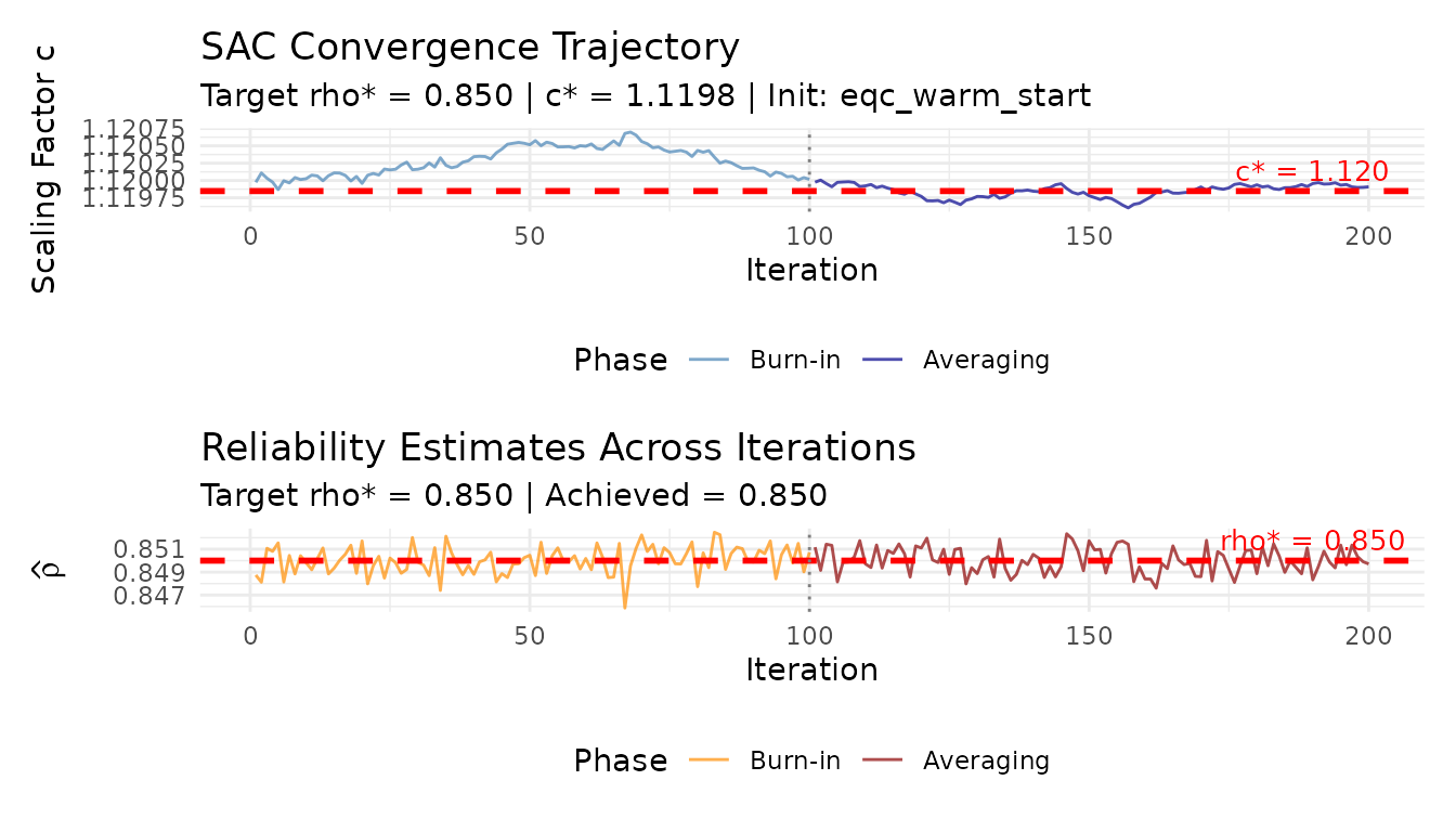

2.4.2 Visualize SAC convergence

plot(sac_result)

SAC convergence diagnostic plot for the warm-start validation run.

2.4.3 Compare EQC and SAC

comparison <- compare_eqc_sac(eqc_result, sac_result)
#> 
#> =======================================================
#>   EQC vs SAC Comparison
#> =======================================================
#> 
#>   Target reliability  : 0.8500
#>   EQC c*              : 1.119883
#>   SAC c*              : 1.119847
#>   Absolute difference : 0.000035
#>   Percent difference  : 0.00%
#>   EQC achieved rho    : 0.8500
#>   SAC achieved rho    : 0.8501
#>   Comparable           : YES
#>   Agreement (< 5%)    : YES
#>   Agreement status     : evaluated
#>   EQC status          : uniroot_success
#>   SAC status          : ok
#>   SAC status flags    : ok
#>

The comparison reports the absolute and percentage difference in c^* between the two algorithms and applies a 5% diagnostic threshold only after verifying that their estimand and item-design contracts are comparable.

2.4.4 SAC parameter reference

Parameter	Default	Description
`c_init`	`NULL` (APC)	Initial c_0; pass an `eqc_result` for warm start
`n_iter`	`300L`	Total Robbins–Monro iterations
`M_per_iter`	`500L`	MC samples per iteration
`M_pre`	`10000L`	MC samples for pre-calculating \sigma^2_\theta
`burn_in`	`floor(n_iter/2)`	Iterations to discard before averaging
`step_params`	`list(a=1, A=50, gamma=0.67)`	Step-size sequence: a_n = a/(n+A)^\gamma
`resample_items`	`TRUE`	`TRUE`: item-superpopulation target; `FALSE`: one fixed form

EQC always calibrates the one generated form. SAC has two explicit scopes:

With resample_items = FALSE, SAC reuses one form. When c_init is an EQC object and item_source/item_params are omitted, it reuses the exact EQC bank and verifies the same target, model, metric, item count, and form.
With resample_items = TRUE, SAC redraws forms and reports the mean reliability over independent holdout forms. This is an item-superpopulation estimand, so an EQC object is not a comparable warm start; use the automatic initializer or a numeric starting value.

2.5 Step 5: Generate Response Data — `simulate_response_data()`

Once calibration is complete, generate a binary response matrix. The function draws N persons from the specified latent distribution and generates responses using the calibrated item parameters.

sim_data <- simulate_response_data(
  result       = eqc_result,
  n_persons    = 500,
  latent_shape = "normal",
  seed         = 123
)

cat(sprintf("Response matrix: %d persons x %d items\n",
            nrow(sim_data$response_matrix),
            ncol(sim_data$response_matrix)))
#> Response matrix: 500 persons x 25 items
cat(sprintf("Mean proportion correct: %.3f\n",
            mean(sim_data$response_matrix)))
#> Mean proportion correct: 0.502
sim_data$provenance[c("metric", "calibration_status", "status_flags",
                      "item_source", "simulation_seed", "latent_shape")]
#> $metric
#> [1] "info"
#> 
#> $calibration_status
#> [1] "uniroot_success"
#> 
#> $status_flags
#> [1] "uniroot_success"
#> 
#> $item_source
#> [1] "parametric"
#> 
#> $simulation_seed
#> [1] 123
#> 
#> $latent_shape
#> [1] "normal"

2.5.1 Inspect the generated data

# First 5 persons, first 5 items
sim_data$response_matrix[1:5, 1:5]
#>      item1 item2 item3 item4 item5
#> [1,]     0     1     0     1     0
#> [2,]     0     1     0     1     1
#> [3,]     1     1     1     1     1
#> [4,]     1     0     0     1     0
#> [5,]     1     0     0     0     1

# Distribution of total scores
total_scores <- rowSums(sim_data$response_matrix)
summary(total_scores)
#>    Min. 1st Qu.  Median    Mean 3rd Qu.    Max. 
#>    0.00    8.00   13.00   12.56   16.00   25.00

hist(total_scores, breaks = 20, col = "steelblue",
     border = "white", main = "Distribution of Total Scores",
     xlab = "Total Score", ylab = "Frequency")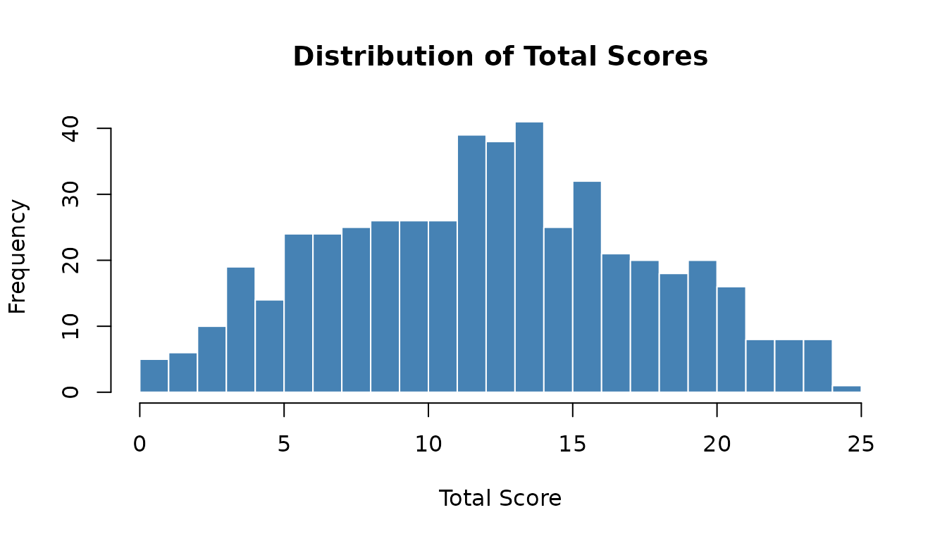

Histogram of total scores from the simulated response matrix.

2.5.2 Classical item analysis

A quick sanity check: compute item-total correlations and item difficulty (proportion correct) from the generated data.

p_correct <- colMeans(sim_data$response_matrix)
item_total_cor <- apply(sim_data$response_matrix, 2, function(x) {
  cor(x, total_scores - x)  # corrected item-total correlation
})

par(mfrow = c(1, 2))
hist(p_correct, breaks = 15, col = "steelblue", border = "white",
     main = "Item Difficulty (p)", xlab = "Proportion Correct")
hist(item_total_cor, breaks = 15, col = "darkorange", border = "white",
     main = "Item-Total Correlation", xlab = "Corrected r_it")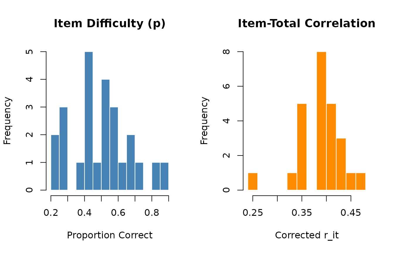

Scatter plot of item difficulty against observed proportion correct in the simulated data.

par(mfrow = c(1, 1))

2.5.3 External validation with TAM

If you have the TAM package installed, you can verify that the achieved reliability provides a useful external diagnostic for Rasch/2PL data:

if (requireNamespace("TAM", quietly = TRUE)) {
  tam_rel <- compute_reliability_tam(sim_data$response_matrix, model = "rasch")
  cat(sprintf("Target reliability: %.4f\n", eqc_result$target_rho))
  cat(sprintf("EQC achieved rho:   %.4f\n", eqc_result$achieved_rho))
  cat(sprintf("TAM WLE reliability: %.4f\n", tam_rel$rel_wle))
  cat(sprintf("TAM EAP reliability: %.4f\n", tam_rel$rel_eap))
}

Note on WLE vs EAP reliability. In many practical TAM fits, EAP reliability is higher than WLE reliability, but EAPrel() and WLErel() use different estimators and variance bases. Inspect both as complementary external diagnostics rather than formal lower/upper bounds.

For 3PL data, fit TAM::tam.mml.3pl() directly and use its EAP person output or EAP.rel only. compute_reliability_tam() intentionally exposes the Rasch/2PL helper contract, and TAM::tam.wle() was unsupported for a tam.mml.3pl object in the validated TAM version. Moreover, EAP score reliability is estimator-, sample-, prior-, and fit-dependent; it is not the same estimand as IRTsimrel’s analytic population information reliability.

2.6 Step 6: Extract and Use Results

2.6.1 `coef()` — calibrated item parameters

The coef() method extracts a tidy data frame of item parameters:

item_df <- coef(eqc_result)
head(item_df)
#>   item_id         beta lambda_base lambda_scaled   c_star
#> 1       1  0.197732269           1      1.119883 1.119883
#> 2       2  1.096799859           1      1.119883 1.119883
#> 3       3  0.436545084           1      1.119883 1.119883
#> 4       4 -0.013038730           1      1.119883 1.119883
#> 5       5 -0.199801302           1      1.119883 1.119883
#> 6       6  0.007700326           1      1.119883 1.119883

Each row contains:

item_id: item identifier.
beta: item difficulty.
lambda_base: baseline (unscaled) discrimination.
lambda_scaled: calibrated discrimination (\lambda_{\text{base}} \times c^*).
c_star: the calibrated scaling factor (constant across items).

2.6.2 `predict()` — reliability at new scaling factors

Use predict() to evaluate reliability at arbitrary scaling factor values:

# Achieved reliability
predict(eqc_result)
#> [1] 0.8500004

# Reliability at several c values
predict(eqc_result, newdata = c(0.5, 1.0, 1.5, 2.0))
#>     c=0.5     c=1.0     c=1.5     c=2.0 
#> 0.5896711 0.8259511 0.8972175 0.9280310

This is useful for sensitivity analysis—for instance, exploring how much reliability changes if the scaling factor shifts by \pm 10\%.

2.6.3 `as.data.frame()` — export item parameters

For downstream analysis, export the calibrated item parameters to a data frame:

items_df <- as.data.frame(eqc_result$items_calib)
head(items_df)
#>   form_id item_id         beta   lambda lambda_unscaled
#> 1       1       1  0.197732269 1.119883               1
#> 2       1       2  1.096799859 1.119883               1
#> 3       1       3  0.436545084 1.119883               1
#> 4       1       4 -0.013038730 1.119883               1
#> 5       1       5 -0.199801302 1.119883               1
#> 6       1       6  0.007700326 1.119883               1

2.6.4 Accessing internal components

The calibration result objects store additional information for advanced use:

# EQC components
cat("EQC result components:\n")
#> EQC result components:
cat(paste(" ", names(eqc_result), collapse = "\n"), "\n\n")
#>   c_star
#>   target_rho
#>   achieved_rho
#>   metric
#>   model
#>   n_items
#>   M
#>   theta_quad
#>   theta_var
#>   beta_vec
#>   lambda_base
#>   lambda_scaled
#>   items_base
#>   items_calib
#>   call
#>   misc
#>   guessing_vec
#>   schema_version
#>   item_scope
#>   estimand_signature
#>   design_signature

# Calibrated scaling factor
cat(sprintf("c* = %.4f\n", eqc_result$c_star))
#> c* = 1.1199

# Latent variance from quadrature sample
cat(sprintf("theta_var = %.4f\n", eqc_result$theta_var))
#> theta_var = 1.0099

2.7 Compact End-to-End 3PL Workflow

A 3PL form has lower asymptotes g_i in addition to difficulty and discrimination:

P(Y_i=1\mid\theta)=g_i+(1-g_i) \operatorname{logit}^{-1}\{c\lambda_{i,0}(\theta-\beta_i)\}.

guessing_params controls g_i. The global scale c multiplies only the baseline discriminations \lambda_{i,0}; it never multiplies the guessing parameters. The next executable example makes that separation explicit and freezes the generated form before calibration.

generated_3pl <- sim_item_params(
  n_items = 12,
  model = "3pl",
  source = "parametric",
  method = "copula",
  guessing_params = list(distribution = "fixed", value = 0.20),
  scale = 1,
  seed = 310
)

fixed_3pl_spec <- list(custom_params = list(
  beta = generated_3pl$data$beta,
  lambda = generated_3pl$data$lambda_unscaled,
  guessing = generated_3pl$data$guessing
))

EQC estimates a discrimination scale for that fixed form. The smaller quadrature setting below is suitable for documentation; increase M and use independent seeded holdouts for a final study.

eqc_3pl <- eqc_calibrate(
  target_rho = 0.70,
  n_items = 12,
  model = "3pl",
  item_source = "custom",
  item_params = fixed_3pl_spec,
  reliability_metric = "info",
  M = 2000L,
  seed = 310
)

coef(eqc_3pl)[1:6, c(
  "beta", "lambda_base", "lambda_scaled", "guessing", "c_star"
)]
#>         beta lambda_base lambda_scaled guessing   c_star
#> 1 -1.1690253   1.0633685      1.258095      0.2 1.183123
#> 2  0.9058676   0.9813886      1.161103      0.2 1.183123
#> 3  0.2164509   1.5745857      1.862928      0.2 1.183123
#> 4  0.7229356   1.3660700      1.616228      0.2 1.183123
#> 5  1.8519541   0.8899961      1.052975      0.2 1.183123
#> 6 -0.7876383   1.2991184      1.537017      0.2 1.183123

For a same-estimand stochastic check, set resample_items = FALSE and omit item-generation arguments. SAC then reuses the exact EQC bank and rejects a mismatched metric or form instead of silently comparing unlike designs.

sac_3pl <- sac_calibrate(
  target_rho = 0.70,
  n_items = 12,
  model = "3pl",
  reliability_metric = "info",
  c_init = eqc_3pl,
  resample_items = FALSE,
  n_iter = 60L,
  M_per_iter = 250L,
  M_pre = 1000L,
  evaluation_controls = list(n_forms = 3L, M = 500L),
  seed = 310
)

same_form_check <- compare_eqc_sac(eqc_3pl, sac_3pl)
#> 
#> =======================================================
#>   EQC vs SAC Comparison
#> =======================================================
#> 
#>   Target reliability  : 0.7000
#>   EQC c*              : 1.183123
#>   SAC c*              : 1.171030
#>   Absolute difference : 0.012093
#>   Percent difference  : 1.02%
#>   EQC achieved rho    : 0.7000
#>   SAC achieved rho    : 0.7045
#>   Comparable           : YES
#>   Agreement (< 5%)    : YES
#>   Agreement status     : evaluated
#>   EQC status          : uniroot_success
#>   SAC status          : ok
#>   SAC status flags    : ok
#> 
stopifnot(same_form_check$comparable)

Finally, generate responses from the calibrated form and verify its structural contract. simulate_response_data() preserves the calibrated discriminations, the fixed lower asymptotes, and provenance.

sim_3pl <- simulate_response_data(
  result = eqc_3pl,
  n_persons = 200,
  seed = 311
)

stopifnot(
  identical(dim(sim_3pl$response_matrix), c(200L, 12L)),
  all(sim_3pl$response_matrix %in% 0:1),
  all(sim_3pl$guessing == 0.20),
  identical(sim_3pl$provenance$item_scope, "fixed_form")
)
c(
  eqc_rho = eqc_3pl$achieved_rho,
  sac_holdout_rho = sac_3pl$achieved_rho,
  response_rate = mean(sim_3pl$response_matrix)
)
#>         eqc_rho sac_holdout_rho   response_rate 
#>       0.7000000       0.7045106       0.5900000

For an item-superpopulation target, use SAC without an EQC-object warm start:

sac_3pl_population <- sac_calibrate(
  target_rho = 0.70,
  n_items = 12,
  model = "3pl",
  item_params = list(
    guessing_params = list(distribution = "fixed", value = 0.20)
  ),
  reliability_metric = "info",
  c_init = NULL,
  resample_items = TRUE,
  n_iter = 300L,
  M_per_iter = 1000L,
  M_pre = 10000L,
  seed = 310
)

Its achieved_rho is the mean over independent holdout-form reliabilities, not the reliability of the single representative form stored for convenient response generation. Setting every g_i=0 recovers exact 2PL behavior in the shared probability and information kernels; existing Rasch/2PL calls remain valid without any new arguments.

3. Choosing EQC vs SAC

The following decision table helps you choose between the two algorithms.

Criterion	EQC (Algorithm 1)	SAC (Algorithm 2)
Speed	Fast (adaptive topology scan plus local root polishing)	Slower (preflight plus iterative updates)
Default metric	\tilde{\rho} (info)	\bar{w} (msem)
Deterministic?	Conditional on the frozen Monte Carlo design	No (stochastic)
Topology contract	Maps the full requested log-scale interval, enumerates crossings/extrema, and applies `root_policy`; no global monotonicity assumption	Preflight must resolve a feasible increasing branch before updates
Can target \bar{w}?	No; use `"info"` / `"tilde"`	Yes, natively
Warm start	Not needed	Compatible EQC object for a same-metric fixed-form run; numeric scale otherwise
Use for validation	Primary calibration	Same-estimand check with `reliability_metric = "info"`
Diagnostics	Root topology, selected branch, and empirical residual	Trajectory, branch, projection, holdout, and Polyak-average diagnostics

Practical recommendation:

Start with EQC using reliability_metric = "info". This is fast and reproducible with a fixed seed and stored form/quadrature design.
Use SAC with reliability_metric = "info" to validate EQC when you want a stochastic same-estimand check.
Use SAC with reliability_metric = "msem" separately when your research question targets \bar{w} directly.
Warm-start fixed-form SAC from EQC when comparing the same form and metric. Do not use an EQC-object warm start for an item-superpopulation run.

4. Choosing the Reliability Metric: info vs msem

IRTsimrel supports two population reliability definitions.

4.1 Average-information reliability (rho-tilde)

\tilde{\rho}(c) = \frac{\sigma^2_\theta \, \bar{\mathcal{J}}(c)} {\sigma^2_\theta \, \bar{\mathcal{J}}(c) + 1}

where \bar{\mathcal{J}}(c) = \mathbb{E}_G[\mathcal{J}(\theta; c)] is the average test information across the latent distribution.

Properties:

Often well behaved on practical intervals, but saturation can create an interior maximum, multiple crossings, or boundary-only feasibility. EQC maps the requested interval adaptively and selects among detected roots with an explicit root_policy.
Upper bound on \bar{w} via Jensen’s inequality.
Faster to compute than \bar{w}.

4.2 MSEM-based marginal reliability (w-bar)

\bar{w}(c) = \frac{\sigma^2_\theta} {\sigma^2_\theta + \mathbb{E}_G[1/\mathcal{J}(\theta; c)]}

Properties:

MSEM-based reliability using the reciprocal-information approximation to conditional error variance.
Can be non-monotone in c for extreme scaling.
Requires SAC for safe targeting.

4.3 Jensen’s inequality: the key relationship

By Jensen’s inequality applied to the convex function f(x) = 1/x:

\mathbb{E}\!\left[\frac{1}{\mathcal{J}(\theta)}\right] \;\geq\; \frac{1}{\mathbb{E}[\mathcal{J}(\theta)]}

which implies \tilde{\rho} \geq \bar{w}. The gap is small when test information is approximately constant across \theta, and larger when information varies substantially (e.g., short tests, non-normal populations).

4.4 Decision guidance

Scenario	Recommended metric	Reason
Standard simulation study	`"info"`	Stable on practical intervals; fast seeded root-finding
MSEM-based marginal reliability needed	`"msem"` via SAC	Uses reciprocal-information error variance
Non-normal latent distribution	`"info"` for EQC	Bracket-checked seeded root-finding
EQC/SAC validation	`"info"` for both	Compare the same estimand via `compare_eqc_sac()`

# Compare metrics for the same calibration
eqc_info <- eqc_calibrate(
  target_rho = 0.85, n_items = 25, model = "rasch",
  reliability_metric = "info", M = 5000L, seed = 42
)

cat(sprintf("Targeting info:  c* = %.4f, achieved = %.4f\n",
            eqc_info$c_star, eqc_info$achieved_rho))
#> Targeting info:  c* = 1.1199, achieved = 0.8500

5. Working with Different Models

5.1 Rasch model

In the Rasch model, all baseline discriminations are equal to 1. The calibrated discriminations are \lambda_i^* = c^* \times 1 = c^* for all items.

eqc_rasch <- eqc_calibrate(
  target_rho  = 0.80,
  n_items     = 20,
  model       = "rasch",
  item_source = "parametric",
  reliability_metric = "info",
  M           = 5000L,
  seed        = 42
)

items_rasch <- coef(eqc_rasch)
cat(sprintf("All lambda_scaled equal? %s\n",
            all(items_rasch$lambda_scaled == items_rasch$lambda_scaled[1])))
#> All lambda_scaled equal? TRUE
cat(sprintf("Common discrimination: %.4f\n", items_rasch$lambda_scaled[1]))
#> Common discrimination: 1.0183

5.2 Two-parameter logistic (2PL) model

In the 2PL model, baseline discriminations vary across items. The scaling factor c^* is applied uniformly:

\lambda_i^* = c^* \times \lambda_{i,0}

eqc_2pl_demo <- eqc_calibrate(
  target_rho  = 0.80,
  n_items     = 25,
  model       = "2pl",
  item_source = "parametric",
  reliability_metric = "info",
  M           = 5000L,
  seed        = 42
)

items_2pl <- coef(eqc_2pl_demo)
cat(sprintf("c* = %.4f\n", eqc_2pl_demo$c_star))
#> c* = 0.8637
cat(sprintf("lambda_scaled range: [%.3f, %.3f]\n",
            min(items_2pl$lambda_scaled), max(items_2pl$lambda_scaled)))
#> lambda_scaled range: [0.460, 1.800]

5.3 Three-parameter logistic (3PL) model

The 3PL retains the varying baseline discrimination of the 2PL and adds a lower asymptote. Reliability calibration changes the common discrimination scale while preserving each item’s difficulty and guessing parameter.

eqc_3pl_demo <- eqc_calibrate(
  target_rho = 0.70,
  n_items = 12,
  model = "3pl",
  item_source = "parametric",
  item_params = list(
    guessing_params = list(distribution = "uniform", min = 0.15, max = 0.25)
  ),
  reliability_metric = "info",
  M = 2000L,
  seed = 42
)

items_3pl_demo <- coef(eqc_3pl_demo)
range(items_3pl_demo$guessing)
#> [1] 0.1500383 0.2439143
stopifnot(all.equal(
  items_3pl_demo$lambda_scaled,
  eqc_3pl_demo$c_star * items_3pl_demo$lambda_base
))

Because nonzero guessing changes the information curve topology, a 3PL calibration can have more than one candidate crossing on a wide scale range. IRTsimrel scans the bounded scale interval and, by default, selects the lowest increasing root. Inspect the stored topology/status instead of assuming that endpoint monotonicity is sufficient.

5.4 Rasch vs 2PL comparison

targets <- c(0.70, 0.75, 0.80, 0.85, 0.90)
comp_df <- data.frame(
  target  = targets,
  c_rasch = numeric(length(targets)),
  c_2pl   = numeric(length(targets))
)

for (i in seq_along(targets)) {
  r1 <- eqc_calibrate(target_rho = targets[i], n_items = 25, model = "rasch",
                       item_source = "parametric", reliability_metric = "info",
                       M = 5000L, seed = 42)
  r2 <- eqc_calibrate(target_rho = targets[i], n_items = 25, model = "2pl",
                       item_source = "parametric", reliability_metric = "info",
                       M = 5000L, seed = 42)
  comp_df$c_rasch[i] <- round(r1$c_star, 4)
  comp_df$c_2pl[i]   <- round(r2$c_star, 4)
}

comp_df
#>   target c_rasch  c_2pl
#> 1   0.70  0.6548 0.6229
#> 2   0.75  0.7572 0.7235
#> 3   0.80  0.8995 0.8637
#> 4   0.85  1.1199 1.0812
#> 5   0.90  1.5328 1.4887

5.5 How latent shape affects calibration

Different latent distribution shapes require different scaling factors to achieve the same target reliability, even with the same item parameters. This is because the test information function interacts differently with each shape.

shapes <- c("normal", "bimodal", "skew_pos", "heavy_tail", "uniform")
shape_df <- data.frame(
  shape      = shapes,
  c_star     = numeric(length(shapes)),
  achieved   = numeric(length(shapes))
)

for (i in seq_along(shapes)) {
  ri <- eqc_calibrate(
    target_rho = 0.80, n_items = 25, model = "rasch",
    latent_shape = shapes[i], item_source = "parametric",
    reliability_metric = "info", M = 5000L, seed = 42
  )
  shape_df$c_star[i]   <- round(ri$c_star, 4)
  shape_df$achieved[i] <- round(ri$achieved_rho, 4)
}

shape_df
#>        shape c_star achieved
#> 1     normal 0.8995      0.8
#> 2    bimodal 0.9577      0.8
#> 3   skew_pos 0.9132      0.8
#> 4 heavy_tail 0.9365      0.8
#> 5    uniform 0.9012      0.8

barplot(
  shape_df$c_star,
  names.arg = shape_df$shape,
  col = "steelblue", border = "white",
  main = "Calibrated c* by Latent Shape (target rho = 0.80)",
  ylab = expression(c^"*"), las = 2, cex.names = 0.8
)
abline(h = mean(shape_df$c_star), lty = 2, col = "grey40")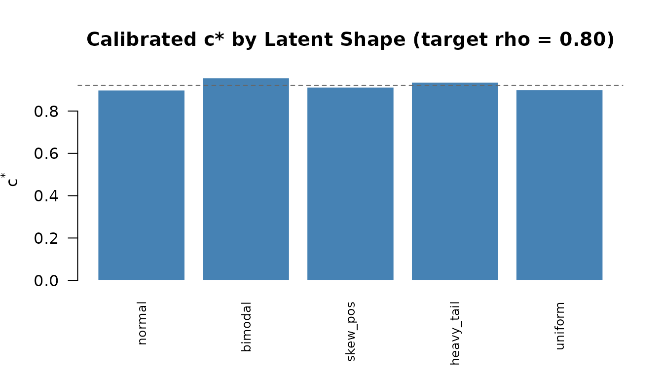

Bar plot comparing achieved reliability across latent distribution shapes.

The barplot reveals that heavy-tailed and skewed distributions generally require higher scaling factors (stronger discriminations) to achieve the same reliability. This makes intuitive sense: extreme \theta values receive less test information under the logistic model, and heavier tails put more mass in those regions.

5.6 Effect of test length on reliability curve

lengths_to_plot <- c(10, 20, 30, 50)
cols <- c("firebrick", "darkorange", "steelblue", "forestgreen")
c_grid <- seq(0.2, 4, length.out = 40)

plot(NULL, xlim = c(0.2, 4), ylim = c(0, 1),
     xlab = "Scaling factor c", ylab = expression(tilde(rho)),
     main = "Reliability Curves by Test Length")
abline(h = 0.80, lty = 2, col = "grey50")

for (j in seq_along(lengths_to_plot)) {
  cd <- rho_curve(
    c_values = c_grid, n_items = lengths_to_plot[j],
    model = "rasch", latent_shape = "normal",
    item_source = "parametric", metric = "info",
    M = 5000L, seed = 42, plot = FALSE
  )
  lines(cd$c, cd$rho_tilde, col = cols[j], lwd = 2)
}

legend("bottomright",
       legend = paste0("I = ", lengths_to_plot),
       col = cols, lwd = 2, bty = "n")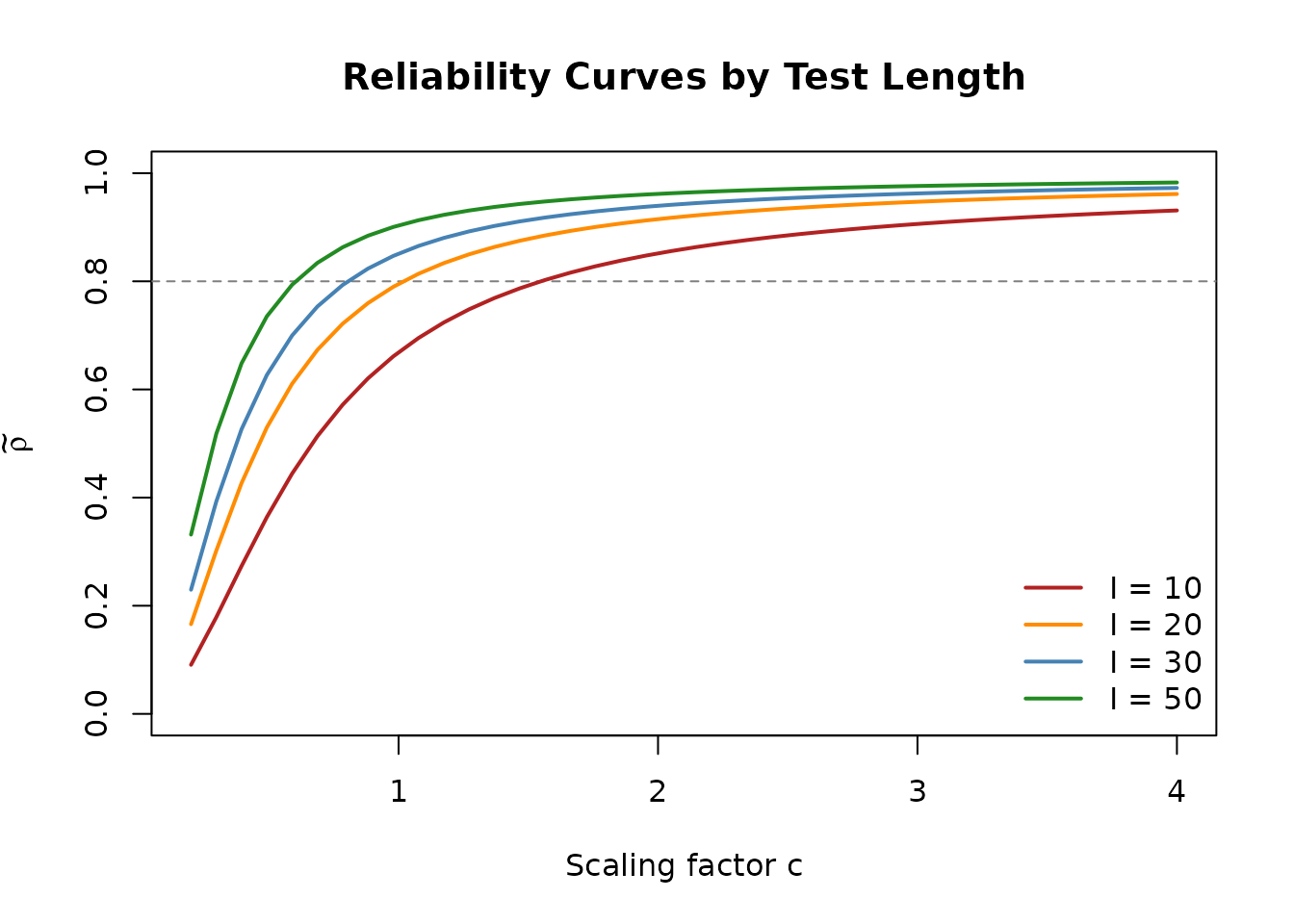

Reliability curves comparing how test length affects the discrimination scale needed for a target reliability.

The figure illustrates a key relationship: longer tests reach any given reliability target at a lower scaling factor. This means that adding items is an alternative to increasing discrimination when a high reliability is needed.

6. Troubleshooting Guide

6.1 Common issues and solutions

“Target reliability not achievable”

Symptom: check_feasibility() shows the target is outside the achievable range.

Solutions:

Increase the number of items.
Switch from Rasch to 2PL (varying discriminations provide more flexibility).
For 3PL designs, inspect the selected root topology and reconsider the guessing distribution or scale bounds rather than assuming monotonicity.
Widen c_bounds in check_feasibility() to explore a larger range.
Consider whether the latent shape makes the target unrealistic.

`uniroot()` fails with “values at endpoints not of opposite sign”

Symptom: EQC calibration fails because the target lies outside the range [\rho(c_{\min}), \rho(c_{\max})].

Solutions:

Run check_feasibility() first.
Widen c_bounds in eqc_calibrate().
If targeting "msem", switch to "info" (the bracket-checked EQC metric).

SAC does not converge

Symptom: The SAC trajectory oscillates without settling.

Solutions:

Increase n_iter (e.g., from 300 to 500 or more).
Decrease the step-size base a in step_params.
Increase A in step_params for more stabilization.
Use a warm start from EQC.
Increase M_per_iter to reduce per-iteration variance.

Results differ between EQC and SAC

Symptom: compare_eqc_sac() reports more than 5% difference.

Possible causes:

Different reliability metrics (check metric field).
Different item scopes (fixed form versus item superpopulation) or item banks.
Insufficient Monte Carlo samples (M for EQC, M_per_iter/n_iter for SAC).
Different random seeds producing different item/theta draws.

Solutions:

Increase M and M_per_iter.
Use reliability_metric = "info" for both algorithms for fair comparison.
For a fixed-form comparison, pass the EQC result with resample_items = FALSE and omit item-generation arguments so the same form is reused. A shared seed alone does not make different estimands comparable.

6.2 Performance tips

Goal	Recommendation
Fast exploration	Use `M = 5000L`, `n_iter = 100L`
Higher-precision starting point	Try `M = 50000L`, `n_iter = 500L`, then verify seed and holdout sensitivity
Quick feasibility check	Use `check_feasibility()` with `M = 3000L`
Reduce SAC variance	Increase `M_per_iter` to 1000 or 2000
Faster SAC	Warm start from EQC, reduce `n_iter`

7. Complete Template: Copy-Paste Workflow

The following code block is a self-contained template you can copy into your project. Replace the settings in the “Configuration” section with your own.

# ============================================================
# Reliability-Targeted IRT Simulation: Complete Workflow
# ============================================================
library(IRTsimrel)

# --- Configuration ------------------------------------------
target_rho   <- 0.85       # desired marginal reliability
n_items      <- 25         # test length
model        <- "rasch"    # "rasch", "2pl", or "3pl"
latent_shape <- "normal"   # latent distribution shape
item_source  <- "parametric"
item_params  <- if (model == "3pl") {
  list(guessing_params = list(distribution = "fixed", value = 0.20))
} else {
  list()
}
N_persons    <- 500        # sample size for response data
M_quad       <- 5000L      # Monte Carlo samples for EQC
seed_val     <- 42         # for reproducibility

# --- Step 1: Feasibility ------------------------------------
feas <- check_feasibility(
  n_items = n_items, model = model,
  latent_shape = latent_shape, item_source = item_source,
  item_params = item_params,
  target_rho = target_rho, M = M_quad, seed = seed_val, verbose = FALSE
)
stopifnot(
  identical(feas$target_status_info_canonical, "feasible"),
  feas$admissible_root_count_info > 0L
)
cat("Step 1: Feasible target with an admissible root confirmed.\n")

# --- Step 2: Reliability curve (optional) --------------------
curve_df <- rho_curve(
  n_items = n_items, model = model,
  latent_shape = latent_shape, item_source = item_source,
  item_params = item_params,
  M = M_quad, seed = seed_val, plot = FALSE
)

# --- Step 3: EQC calibration --------------------------------
eqc_res <- eqc_calibrate(
  target_rho = target_rho, n_items = n_items,
  model = model, latent_shape = latent_shape,
  item_source = item_source,
  item_params = item_params,
  reliability_metric = "info",
  M = M_quad, seed = seed_val
)
cat(sprintf("Step 3: EQC calibrated c* = %.4f, achieved rho = %.4f\n",
            eqc_res$c_star, eqc_res$achieved_rho))

# --- Step 4: SAC validation (optional) ----------------------
sac_res <- sac_calibrate(
  target_rho = target_rho, n_items = n_items,
  model = model, latent_shape = latent_shape,
  reliability_metric = "info",
  c_init = eqc_res,
  resample_items = FALSE,
  n_iter = 200L, M_per_iter = 500L, M_pre = 5000L,
  seed = seed_val
)
cat(sprintf("Step 4: SAC calibrated c* = %.4f\n", sac_res$c_star))

# --- Step 5: Generate response data -------------------------
sim_data <- simulate_response_data(
  result = eqc_res, n_persons = N_persons,
  latent_shape = latent_shape, seed = 123
)
cat(sprintf("Step 5: Generated %d x %d response matrix.\n",
            nrow(sim_data$response_matrix),
            ncol(sim_data$response_matrix)))

# --- Step 6: Extract results --------------------------------
item_params <- coef(eqc_res)
cat(sprintf("Step 6: Extracted %d item parameters.\n", nrow(item_params)))

8. Publication-Ready Language

The following text templates can be adapted for the Method section of a journal paper. Replace bracketed values with your specific settings.

8.1 Describing the simulation design

Item response data were generated using the reliability-targeted simulation framework of Lee (2026), implemented in the R package IRTsimrel (version 0.3.0). A [Rasch / two-parameter logistic / three-parameter logistic] model was assumed with [25] items and latent abilities drawn from a [standard normal / bimodal / skewed] distribution. For the 3PL, item lower asymptotes were [fixed at 0.20 / generated from the stated distribution], and calibration multiplied discrimination only.

8.2 Describing the calibration

The global discrimination scaling factor c^* was calibrated using the Empirical Quadrature Calibration algorithm (EQC; Algorithm 1 in Lee, 2026) with a Monte Carlo quadrature sample of size M = [10,000] and the average-information reliability metric (\tilde{\rho}). The target marginal reliability was set to \rho^* = [0.85], and the achieved reliability was [0.8500].

8.3 Describing optional SAC validation

EQC results were cross-validated using the Stochastic Approximation Calibration algorithm (SAC; Algorithm 2 in Lee, 2026) with [300] Robbins–Monro iterations, warm-started from the EQC solution. The two algorithms agreed to within [X]% on the calibrated scaling factor.

8.4 Describing the response data

Binary item response data were generated for N = [500] simulated examinees using the calibrated item parameters. Each response Y_{pi} was drawn from \text{Bernoulli}(p_{pi}) where p_{pi} = g_i + (1-g_i) \text{logit}^{-1}[\lambda_i^*(\theta_p - \beta_i)] (with g_i=0 for Rasch/2PL). Simulation provenance, including metric, calibration status, item source, latent shape, and seed, was retained with each generated data object.

8.5 Citing the package

Lee, J.-H. (2026). Reliability-Targeted Simulation of Item Response Data: Solving the Inverse Design Problem. arXiv:2512.16012v2. https://doi.org/10.48550/arXiv.2512.16012

9. Further Reading

The IRTsimrel documentation suite includes several companion vignettes:

vignette("quick-start") — A minimal 5-minute introduction.
vignette("latent-distributions") — Detailed guide to all 12 latent distribution shapes and the pre-standardization principle.
vignette("item-parameters") — Sources and methods for generating realistic item parameters, including the copula method and optional IRW integration.
vignette("theory-reliability") — Mathematical foundations of \tilde{\rho} and \bar{w}.
vignette("algorithm-eqc") — Detailed derivation and analysis of Algorithm 1.
vignette("algorithm-sac") — Detailed derivation and analysis of Algorithm 2.
vignette("validation") — Comprehensive validation studies comparing IRTsimrel outputs against TAM.
vignette("api-reference") — Complete function reference with all parameters.

References

Lee, J.-H. (2026). Reliability-Targeted Simulation of Item Response Data: Solving the Inverse Design Problem. arXiv:2512.16012v2. https://doi.org/10.48550/arXiv.2512.16012

Robbins, H., & Monro, S. (1951). A stochastic approximation method. The Annals of Mathematical Statistics, 22(3), 400–407.

Polyak, B. T., & Juditsky, A. B. (1992). Acceleration of stochastic approximation by averaging. SIAM Journal on Control and Optimization, 30(4), 838–855.

Baker, F. B., & Kim, S.-H. (2004). Item Response Theory: Parameter Estimation Techniques (2nd ed.). Marcel Dekker.

Sweeney, S. M., et al. (2022). An investigation of the nature and consequence of the relationship between IRT difficulty and discrimination. Educational Measurement: Issues and Practice, 41(4), 50–67.

JoonHo Lee (jlee296@ua.edu)

2026-08-22

1. Overview

2. The 6-Step Workflow

2.1 Step 1: Screen Feasibility with check_feasibility()

Comparing feasibility across designs

2.2 Step 2: Explore the Reliability Curve with rho_curve()

2.3 Step 3: Calibrate with EQC — eqc_calibrate()

2.3.1 Basic calibration (Rasch)

2.3.2 Exploring the result

2.3.3 Key parameters explained

2.3.4 Calibrating under different models and shapes

2.4 Step 4: (Optional) Validate with SAC — sac_calibrate()

2.4.1 Warm-start from EQC (recommended)

2.4.2 Visualize SAC convergence

2.4.3 Compare EQC and SAC

2.4.4 SAC parameter reference

2.5 Step 5: Generate Response Data — simulate_response_data()

2.5.1 Inspect the generated data

2.5.2 Classical item analysis

2.5.3 External validation with TAM

2.6 Step 6: Extract and Use Results

2.6.1 coef() — calibrated item parameters

2.6.2 predict() — reliability at new scaling factors

2.6.3 as.data.frame() — export item parameters

2.6.4 Accessing internal components

2.7 Compact End-to-End 3PL Workflow

3. Choosing EQC vs SAC

4. Choosing the Reliability Metric: info vs msem

4.1 Average-information reliability (rho-tilde)

4.2 MSEM-based marginal reliability (w-bar)

4.3 Jensen’s inequality: the key relationship

4.4 Decision guidance

5. Working with Different Models

5.1 Rasch model

5.2 Two-parameter logistic (2PL) model

5.3 Three-parameter logistic (3PL) model

5.4 Rasch vs 2PL comparison

5.5 How latent shape affects calibration

5.6 Effect of test length on reliability curve

6. Troubleshooting Guide

6.1 Common issues and solutions

“Target reliability not achievable”

uniroot() fails with “values at endpoints not of opposite sign”

SAC does not converge

Results differ between EQC and SAC

6.2 Performance tips

7. Complete Template: Copy-Paste Workflow

8. Publication-Ready Language

8.1 Describing the simulation design

8.2 Describing the calibration

8.3 Describing optional SAC validation

8.4 Describing the response data

8.5 Citing the package

9. Further Reading

References

2.1 Step 1: Screen Feasibility with `check_feasibility()`

2.2 Step 2: Explore the Reliability Curve with `rho_curve()`

2.3 Step 3: Calibrate with EQC — `eqc_calibrate()`

2.4 Step 4: (Optional) Validate with SAC — `sac_calibrate()`

2.5 Step 5: Generate Response Data — `simulate_response_data()`

2.6.1 `coef()` — calibrated item parameters

2.6.2 `predict()` — reliability at new scaling factors

2.6.3 `as.data.frame()` — export item parameters

`uniroot()` fails with “values at endpoints not of opposite sign”