IRTsimrel: Reliability-Targeted IRT Simulation

JoonHo Lee (jlee296@ua.edu)

2026-08-22

1. Introduction

In Monte Carlo simulation studies for Item Response Theory (IRT), researchers carefully manipulate sample size, test length, item parameter distributions, and latent trait shapes. Yet marginal reliability — the single number that best summarises how informative a test is — is almost never directly controlled. Instead, it emerges as an implicit, unreported consequence of these design choices. The IRTsimrel package closes that gap by letting you specify a target reliability as an explicit input parameter, then calibrating the data-generating process so the simulated test hits that target.

IRTsimrel implements the framework described in Lee (2026). It provides two calibration algorithms (EQC and SAC), a rich set of latent-distribution and item-parameter generators, and diagnostic tools for feasibility screening and reliability visualization. Whether you are running a large-scale Monte Carlo study or generating a single dataset for classroom use, the package gives you principled control over the signal-to-noise ratio in your simulated data.

This introductory vignette is the gateway to the rest of the package documentation. It provides a high-level overview of the core ideas, the two calibration algorithms, the two reliability metrics, and the full set of exported functions. At the end, a reading roadmap helps you find the vignette most relevant to your goals, whether you are an applied researcher who just needs to simulate data, or a methodological researcher who wants to understand the mathematical foundations.

2. The Core Challenge: Why Reliability Matters

2.1 The ICC Analogy

Multilevel modelling (MLM) researchers would never run a simulation study without specifying the intraclass correlation (ICC). The ICC controls the signal-to-noise ratio — the proportion of total variance attributable to the cluster-level random effect versus residual noise. Every credible MLM simulation paper reports and systematically varies ICC as a primary design factor.

Marginal reliability in IRT serves the same conceptual role as ICC in MLM. Both quantities capture the ratio of signal variance to total variance. In IRT the “signal” is the latent trait \theta and the “noise” is measurement error. Despite this parallel, the vast majority of IRT simulation studies never report or control the implied reliability of their simulated data.

Consider how ICC appears in a typical MLM simulation paper: the authors might specify ICC values of 0.05, 0.15, and 0.30, and systematically evaluate how model performance varies across these conditions. By contrast, an IRT simulation paper might specify item discriminations of \lambda = 1.0 and test length of I = 30, but never compute or report the implied reliability of the resulting test. As Lee (2026) argues, this is a serious methodological gap that undermines the interpretability and generalizability of simulation results.

IRTsimrel brings IRT simulation methodology into alignment with this long-standing best practice in multilevel modelling.

2.2 Three Consequences of the “Reliability Omission”

When reliability is left uncontrolled in IRT simulation studies, three interrelated problems follow:

1. Ecological validity threat. Operational assessments commonly have reliabilities between 0.50 and 0.70 (especially short screening instruments, formative assessments, and subscales). However, simulation studies frequently use item parameters that imply reliabilities above 0.90. Conclusions drawn under such optimistic conditions may not generalize to the lower-reliability regime that characterizes many real-world applications. When a researcher reports that a new estimator performs well, the reader has no way of knowing whether the same would hold at \rho = 0.60.

2. Confounded comparisons. Claims that one model or estimator outperforms another may hold only within a narrow reliability regime. Two studies that ostensibly compare the same pair of methods may reach opposite conclusions simply because they used different (and unreported) reliability levels. Without systematically varying reliability as a factor in the simulation design, such conclusions are fragile and potentially misleading.

3. Limited replicability. If the implied reliability is not documented, no other researcher can construct a comparable data-generating process. Even if all item parameter values are reported, subtle choices about the latent distribution shape or the correlation between difficulty and discrimination can change the implied reliability. This undermines the replicability of simulation studies — precisely the domain where replicability should be easiest to achieve.

2.3 A Formal Definition

To fix ideas, consider the average-information marginal reliability, which IRTsimrel targets by default:

\tilde{\rho} \;=\; \frac{\sigma_\theta^2 \,\bar{\mathcal{J}}} {\sigma_\theta^2 \,\bar{\mathcal{J}} + 1}

where \sigma_\theta^2 is the latent trait variance and \bar{\mathcal{J}} = \mathbb{E}_\theta[\mathcal{J}(\theta)] is the marginal (average) test information. Under the package’s fixed logistic convention (D = 1), write

q_i(\theta) = \operatorname{logit}^{-1}\!\left[\lambda_i (\theta-\beta_i)\right], \qquad P_i(\theta) = g_i + (1-g_i)q_i(\theta),

where g_i is the 3PL lower asymptote (zero for Rasch/2PL). Test information is then

\mathcal{J}(\theta) \;=\; \sum_{i=1}^{I} \frac{\{(1-g_i)\lambda_i q_i(\theta)[1-q_i(\theta)]\}^2} {P_i(\theta)[1-P_i(\theta)]}.

For g_i=0, this reduces exactly to \lambda_i^2q_i(\theta)[1-q_i(\theta)]. The formulas make explicit that reliability depends on both the item parameters (through \bar{\mathcal{J}}) and the latent distribution (through \sigma_\theta^2 and the expectation over \theta). Changing either one changes the implied reliability, which is precisely why it must be actively controlled.

The reliability formula has an intuitive interpretation: it is a ratio of signal to total variance, just like ICC. When average test information \bar{\mathcal{J}} is large (high discrimination, many items), most of the variance in observed scores is due to true differences in \theta. When \bar{\mathcal{J}} is small, measurement error dominates.

3. How IRTsimrel Works

3.1 The Key Idea: Separation of Structure and Scale

IRTsimrel decouples two aspects of the data-generating process:

Aspect	What it controls	Source
Structure	Difficulty distribution, discrimination patterns, difficulty–discrimination correlation, latent shape	sim_item_params(), sim_latentG()
Scale	Global discrimination level \Rightarrow overall informativeness \Rightarrow reliability	Calibration via eqc_calibrate() or sac_calibrate()

This separation is the central innovation. Structure captures all the qualitative features of the data-generating process — how difficulties are spread, whether discriminations vary across items, whether the latent distribution is skewed or multimodal. These features come from realistic generators (parametric distributions by default, optional Item Response Warehouse integration when available, or user-supplied custom parameters). Within a fixed form, difficulty, relative discrimination, and 3PL guessing are held fixed while discrimination alone is scaled. In an SAC item-superpopulation run, individual forms are redrawn from the same normalized generator rather than preserved item by item.

The intervention acts only on the overall discrimination scale through a single scaling factor c^*. Given baseline (unscaled) discriminations \lambda_{i,0}, the calibrated discriminations are:

\lambda_i^* \;=\; c^* \cdot \lambda_{i,0}

Increasing c^* always amplifies all discriminations proportionally and preserves their relative structure (for example, the ratio \lambda_2 / \lambda_1). On a detected increasing branch in the regular calibration region, this also raises the targeted reliability. No global direction is assumed outside that branch because response saturation and finite-grid effects can produce extrema or multiple crossings. The calibration algorithm finds a selected-branch value c^* whose empirical quadrature or stochastic reliability estimate matches the user’s target \rho^*. Population-level accuracy is an approximation governed by the Monte Carlo design and should be checked on independent draws.

3.2 How It Works in Practice

The workflow has three steps:

1. Generate structure. Call sim_latentG() to draw latent abilities from a specified distribution, and sim_item_params() to draw item parameters from a specified source. These provide the qualitative “shape” of the data-generating process.

2. Calibrate scale. Call eqc_calibrate() (or sac_calibrate()) with your target reliability. The function uses the generated structure to find a scaling factor c^* whose selected empirical objective matches \rho_{\text{target}}.

3. Generate data. Call simulate_response_data() with the calibration result to produce a binary response matrix from the calibrated design. Finite-sample reliability estimates can differ from the analytic target.

3.3 A Minimal Example

Here is a complete EQC calibration in five lines of code:

# Calibrate a 20-item Rasch test for target reliability 0.80
result <- eqc_calibrate(
  target_rho = 0.80,
  n_items    = 20,
  model      = "rasch",
  item_source = "parametric",
  reliability_metric = "info",
  seed       = 42,
  M          = 5000L
)

# Inspect the calibration result
result
#> 
#> =======================================================
#>   Empirical Quadrature Calibration (EQC) Results
#> =======================================================
#> 
#> Calibration Summary:
#>   Model                        : RASCH
#>   Target reliability (rho*)    : 0.8000
#>   Achieved reliability         : 0.8000
#>   Absolute error               : 1.08e-07
#>   Scaling factor (c*)          : 1.0183
#> 
#> Design Parameters:
#>   Number of items (I)          : 20
#>   Quadrature points (M)        : 5000
#>   Reliability metric           : Average-information (tilde)
#>   Latent variance              : 1.0099
#> 
#> Convergence:
#>   Root status                  : uniroot_success
#>   Calibration status           : ok
#>   Roots detected               : 1
#>   Search bracket               : [0.300, 3.000]
#>   Bracket reliabilities        : [0.3054, 0.9471]
#> 
#> Parameter Summaries:
#>   theta:        mean = -0.014, sd = 1.005
#>   beta:         mean = -0.000, sd = 0.758, range = [-2.15, 1.12]
#>   lambda_base:  mean = 1.000, sd = 0.000
#>   lambda_scaled: mean = 1.018, sd = 0.000

The output reports the calibrated scaling factor c*, the achieved reliability, and topology diagnostics. The reported residual measures agreement on the fixed calibration quadrature. A small residual confirms numerical solution of that empirical objective; it does not by itself establish the same error on an independent population draw.

3.4 From Calibration to Data

With the calibration result in hand, generating response data takes one more call:

# Generate 500 response vectors from the calibrated DGP
sim <- simulate_response_data(
  result    = result,
  n_persons = 500,
  seed      = 123
)

# The result is a 500 x 20 binary matrix
dim(sim$response_matrix)
#> [1] 500  20

sim$provenance[c("metric", "calibration_status", "status_flags", "item_source")]
#> $metric
#> [1] "info"
#> 
#> $calibration_status
#> [1] "uniroot_success"
#> 
#> $status_flags
#> [1] "uniroot_success"
#> 
#> $item_source
#> [1] "parametric"

The response data inherit the calibrated item design, but a finite response sample can have an estimator-specific reliability different from the analytic target. The result also carries provenance metadata describing the metric, calibration status, item source, design, and simulation seed. You can use the response matrix directly in any downstream analysis: model fitting, parameter recovery studies, comparison of estimators, or power analysis.

4. Two Algorithms

IRTsimrel provides two calibration algorithms. EQC targets the average-information metric (reliability_metric = "info"), while SAC defaults to the MSEM-based metric (reliability_metric = "msem") and can also be set to "info" for same-estimand validation. Both algorithms find a scaling factor c^* such that the selected reliability metric equals \rho^*, but they differ in their approach and strengths.

4.1 Algorithm 1: EQC (Empirical Quadrature Calibration)

EQC draws a fixed Monte Carlo sample (“quadrature”) of M abilities and one fixed item form. It adaptively maps the complete user-supplied interval on the log scale, polishes detected local crossings with Brent’s method (uniroot()), and selects an admissible branch according to root_policy.

How it works:

1. Draw \{\theta_m\}_{m=1}^M \sim G and \{(\beta_i, \lambda_{i,0})\}_{i=1}^I \sim H once.
2. For any candidate c, form \lambda_i(c) = c \cdot \lambda_{i,0} and compute the empirical reliability \hat{\rho}_M(c).
3. Enumerate detected crossings, tangencies, plateaus, and extrema; polish bracketed crossings locally and apply the requested root-selection policy.

Strengths: Fast, deterministic conditional on the fixed draw, explicit about root topology, and reproducible with a fixed seed. It is the recommended default for routine fixed-form simulation studies.

When to use EQC:

• Routine simulation studies where you need fast, reliable calibration.
• Rasch, 2PL, or 3PL models with supported item and latent generators.
• As initialization (warm start) for SAC.

4.2 Algorithm 2: SAC (Stochastic Approximation Calibration)

SAC uses the Robbins-Monro stochastic approximation algorithm after a deterministic topology preflight has selected a feasible increasing branch. At each iteration it draws a fresh mini-batch of abilities, computes a noisy reliability estimate, and takes a gradient-like step toward the target. Items are reused for resample_items = FALSE (fixed form) and redrawn for resample_items = TRUE (item-superpopulation). After a burn-in phase, Polyak-Ruppert averaging yields the final estimate c^*.

The update rule:

c_{n+1} \;=\; c_n \;-\; a_n \cdot (\hat{\rho}_n - \rho^*)

where a_n = a / (n + A)^\gamma is a decreasing step size satisfying the Robbins-Monro conditions \sum a_n = \infty and \sum a_n^2 < \infty.

Strengths: Targets \bar{w} directly when initialized on a stable branch, provides convergence diagnostics, works with arbitrary DGPs, and can independently validate EQC results.

When to use SAC:

• Independent validation of EQC results.
• Targeting the MSEM-based reciprocal-information reliability \bar{w}, where the objective may be non-monotone and root-finding can fail.
• Complex data-generating processes where the test information function is not easily evaluated in closed form.

Warm start from EQC: For the best of both worlds, run EQC first, then pass the result to SAC as a warm start. This combines the speed of EQC with the robustness of SAC:

eqc_res <- eqc_calibrate(
  target_rho = 0.80, n_items = 20,
  reliability_metric = "info", ...
)
sac_res <- sac_calibrate(target_rho = 0.80, n_items = 20,
                          reliability_metric = "info",
                          c_init = eqc_res,
                          resample_items = FALSE, ...)

4.3 Decision Guide

Scenario	Recommended	Rationale
Standard Rasch/2PL/3PL fixed form, need quick answer	EQC	Deterministic conditional on the fixed draw; fast and topology-aware
Targeting \tilde{\rho} (average-information)	EQC	Deterministic root-finding with bracket checks
Targeting \bar{w} (MSEM-based)	SAC	Direct stochastic targeting with convergence diagnostics
Validating an EQC result	SAC warm start with reliability_metric = "info"	Independent confirmation of the same estimand
Item-superpopulation target	SAC with resample_items = TRUE	Calibrates and evaluates across independently redrawn forms
Large-scale Monte Carlo study	EQC + optional SAC check	Speed for production, SAC for spot checks

For most users in most situations, EQC is the right choice. Use SAC when you need extra assurance or when the mathematical properties of your specific problem require it.

5. Two Reliability Metrics

IRTsimrel supports two population-level reliability metrics from Lee (2026). Understanding the distinction is important for choosing the right algorithm and interpreting results.

5.1 Average-Information Reliability (rho-tilde)

\tilde{\rho}(c) \;=\; \frac{\sigma_\theta^2 \,\bar{\mathcal{J}}(c)} {\sigma_\theta^2 \,\bar{\mathcal{J}}(c) + 1} \qquad\text{where}\quad \bar{\mathcal{J}}(c) = \mathbb{E}_\theta[\mathcal{J}(\theta;\,c)]

This metric uses the arithmetic mean of the test information function across the latent distribution. It is often well behaved on practical search intervals, but it is not generally linear in c^2: response probabilities also change with c, and saturation can create an interior maximum and multiple crossings. EQC therefore maps the interval, identifies root topology, and applies an explicit branch policy instead of assuming global monotonicity or a unique root.

The compute_rho_tilde() function computes this metric directly from a scaling factor, theta sample, and item parameters. Inside eqc_calibrate(), this is the default metric (reliability_metric = "info").

5.2 MSEM-Based Reliability (w-bar)

\bar{w}(c) \;=\; \frac{\sigma_\theta^2} {\sigma_\theta^2 + \text{MSEM}(c)} \qquad\text{where}\quad \text{MSEM}(c) = \mathbb{E}_\theta\!\left[\frac{1}{\mathcal{J}(\theta;\,c)}\right]

This metric uses the harmonic mean of test information (via the mean squared error of measurement). It is an MSEM-based marginal reliability defined with the asymptotic reciprocal-information approximation to conditional error variance. However, its objective \bar{w}(c) - \rho^* can be non-monotone at extreme scaling factors (see Lee, 2026, Section 4.3), which is why SAC is preferred for targeting \bar{w} directly.

The compute_rho_bar() function computes this metric, and compute_rho_both() computes both metrics in a single pass for efficiency.

5.3 Jensen’s Inequality: rho-tilde >= w-bar

For the same positive information distribution, or the same finite quadrature grid, Jensen’s inequality applied to the convex function f(x) = 1/x implies that the harmonic mean of test information is no greater than the arithmetic mean. This implies:

\tilde{\rho}(c) \;\geq\; \bar{w}(c) \quad \text{for all } c > 0

The gap between the two metrics is small when test information is roughly constant across the latent distribution (e.g., a well-targeted Rasch test with normally distributed abilities) and larger when information varies substantially (e.g., short tests with skewed latent distributions or extreme difficulty values).

5.4 Visualizing the Reliability Curve

The rho_curve() function visualizes both metrics simultaneously as a function of the scaling factor c:

curve_data <- rho_curve(
  n_items = 20,
  model   = "rasch",
  metric  = "both",
  M       = 5000L,
  seed    = 42,
  plot    = TRUE
)

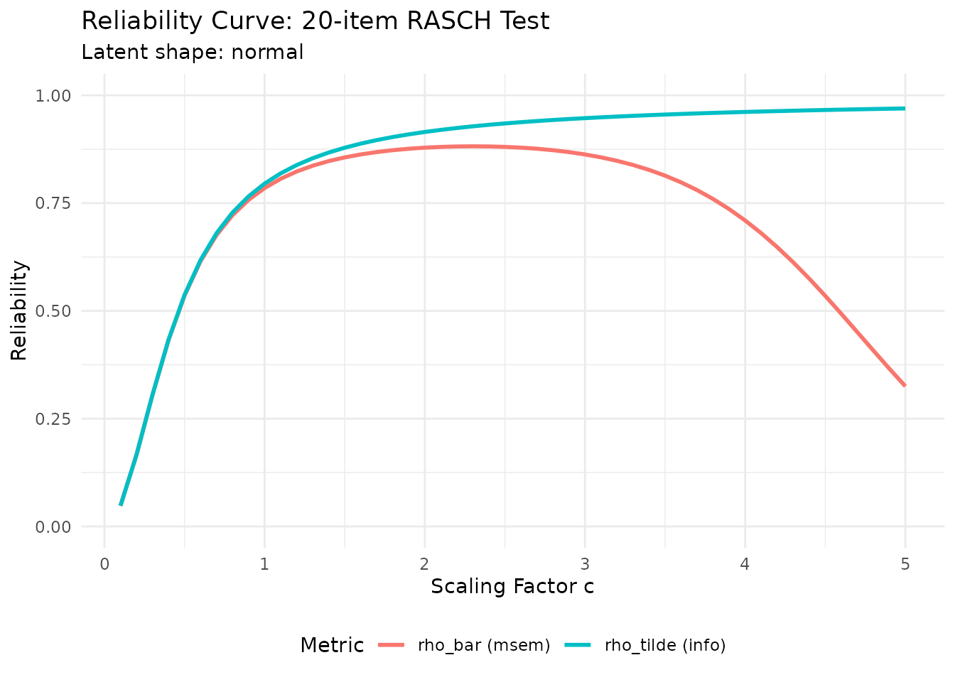
Reliability as a function of the scaling factor c for a 20-item Rasch test. The gap between the two curves reflects Jensen’s inequality on the same quadrature grid: the average-information metric lies above or on the MSEM-based metric.

This plot is useful for several purposes: understanding the feasible range of reliabilities, seeing how sensitive reliability is to the discrimination level, and verifying that the gap between \tilde{\rho} and \bar{w} is small for your particular configuration.

6. What the Package Offers

6.1 Exported Functions

IRTsimrel exports 16 user-facing functions organized into five categories:

Simulation generators:

Function	Purpose
sim_latentG()	Generate latent abilities from a flexible distribution family (12 shapes)
sim_item_params()	Generate item parameters (parametric default, optional IRW, hierarchical, custom sources)
simulate_response_data()	Generate a binary response matrix from a calibration result

Calibration algorithms:

Function	Purpose
eqc_calibrate()	Algorithm 1: adaptive topology scan, explicit branch selection, and local Brent polishing for average-information reliability
sac_calibrate()	Algorithm 2: stochastic calibration via Robbins-Monro approximation

Reliability computation:

Function	Purpose
compute_rho_tilde()	Compute the average-information reliability at a given c
compute_rho_bar()	Compute the MSEM-based marginal reliability at a given c
compute_rho_both()	Compute both metrics in a single matrix pass (performance optimization)
compute_apc_init()	Analytic pre-calibration: closed-form initial value for c

Diagnostics and screening:

Function	Purpose
check_feasibility()	Screen whether a target reliability is achievable for a given design
rho_curve()	Compute and plot \rho(c) over a grid of scaling factor values
compute_reliability_tam()	Rasch/2PL TAM helper returning WLE and EAP diagnostics; direct 3PL TAM validation is EAP-only in the validated workflow

Comparison and visualization:

Function	Purpose
compare_eqc_sac()	Compare EQC and SAC calibration results with the same target, metric, and design
compare_shapes()	Visualize and compare latent distribution shapes

Two deprecated aliases (spc_calibrate() and compare_eqc_spc()) are retained for backward compatibility with code written for v0.1.0.

6.2 S3 Methods

Every core object class has a rich set of S3 methods for inspection and extraction. These make it easy to work with IRTsimrel results using standard R idioms.

latent_G objects (from sim_latentG()):

• print() — concise one-line summary
• summary() — distributional statistics (mean, SD, skewness, kurtosis)
• print.summary() — formatted display of summary
• plot() — density plot of the latent distribution
• as.numeric() — extract raw theta vector

item_params objects (from sim_item_params()):

• print() — concise parameter summary
• summary() — statistics for each parameter type
• print.summary() — formatted display
• plot() — scatterplot of difficulty vs. discrimination
• as.data.frame() — convert to a tidy data frame

eqc_result objects (from eqc_calibrate()):

• print() — full calibration report
• summary() — key results in compact form
• print.summary() — formatted display
• coef() — extract calibrated item parameters as a data frame
• predict() — evaluate reliability at new scaling factor values

sac_result objects (from sac_calibrate()):

• print() — full calibration report with convergence diagnostics
• summary() — key results in compact form
• print.summary() — formatted display
• plot() — convergence trajectory (scaling factor and reliability)
• coef() — extract calibrated item parameters as a data frame
• predict() — evaluate reliability at new scaling factor values

Other classes:

• feasibility_check: print() displays achievable reliability ranges
• rho_curve: print() displays curve summary and first few rows

In total, the package provides 24 S3 methods for interactive exploration of results.

6.3 New in v0.3.0

Version 0.3.0 extends the reliability-targeted workflow while preserving existing Rasch/2PL calls:

• End-to-end 3PL support (D = 1): item generation, analytic probability and information kernels, EQC, SAC, S3 extraction, and response generation now carry lower asymptotes explicitly. The global scale multiplies discrimination only; it never denotes or rescales guessing.

• Topology-aware calibration: feasibility tools and EQC map the complete requested interval, record crossings and extrema, and use an explicit root_policy. This replaces any assumption of a globally monotone curve or a unique root.

• Guarded SAC scopes: deterministic branch preflight precedes stochastic updates. resample_items = FALSE targets a fixed form, whereas TRUE targets an item superpopulation and is evaluated on independent forms.

• Strict warm starts and comparison contracts: EQC-object warm starts and EQC–SAC comparisons check model, metric, item scope, and design provenance instead of comparing scales from incompatible estimands.

• Expanded diagnostics and bounded-memory reducers: result objects retain root/branch, RNG, evaluation, and iteration provenance, while large analytic information calculations are automatically chunked.

The v0.2 diagnostics (check_feasibility(), rho_curve(), compute_rho_both(), and coef()/predict() methods) remain available. The former SPC names are legacy-only deprecated aliases; new code should use SAC terminology.

Here is check_feasibility() in action:

# Screen what reliabilities are achievable for this design
feas <- check_feasibility(
  n_items   = 20,
  model     = "rasch",
  target_rho = 0.80,
  seed      = 42,
  M         = 5000L,
  verbose   = FALSE
)
feas
#> 
#> =======================================================
#>   Feasibility Check: Achievable Reliability Range
#> =======================================================
#> 
#>   Number of items  : 20
#>   Model            : RASCH
#>   Latent shape     : normal
#>   Latent variance  : 1.0099
#>   c range          : [0.10, 10.00]
#>   Monte Carlo M    : 5000
#> 
#> Achievable Reliability Ranges:
#>   rho_tilde (info) : [0.0479, 0.9850]
#>   rho_bar   (msem) : [0.0000, 0.8818]
#> 
#> Target rho*        : 0.8000
#>   info status      : feasible
#>   msem status      : feasible
#> 
#> Note: rho_tilde >= rho_bar on the same information grid (Jensen's inequality).
#>   rho_tilde range screens EQC targets; root policy must still admit a root.
#>   rho_bar range screens SAC targets; stable interior-branch preflight is also required.

The legacy target_status_info and target_status_msem fields locate the target relative to the resolved range. Use target_status_*_canonical to retain an explicit uncertain state when topology is unresolved, and inspect the corresponding admissible-root count before treating range membership as calibration-ready.

7. Road Map to the Vignettes

The IRTsimrel documentation is organized into two parallel tracks so you can find the right level of detail for your needs. All vignettes are accessible from the package website or via vignette("name") in your R console.

7.1 Applied Researchers Track

This track focuses on how to use the package in practice, with emphasis on complete worked examples, actionable guidance, and minimal mathematical detail. If you primarily want to generate data for your simulation study, start here.

Vignette	Title	Est. Time	What You Will Learn
Quick Start	Quick Start	5 min	Calibrate, generate data, and extract results in a single pass
Applied Guide	Applied Guide	30 min	Complete applied tutorial: 2PL models, non-normal distributions, optional IRW items
Latent Distributions	Latent Distributions	20 min	All 12 latent shapes, when to use each, custom mixtures, visualization
Item Parameters	Item Parameters	20 min	Parametric, IRW, hierarchical, and custom item generation, correlated params
Simulation Design	Simulation Design	25 min	Factorial designs with crossed reliability levels, looping over conditions
Case Studies	Case Studies	30 min	Complete worked examples for model comparison, latent misspecification, and sample-size planning

7.2 Methodological Researchers Track

This track covers the mathematical and algorithmic foundations for readers who want to understand or extend what happens under the hood. If you are developing new calibration methods or writing a methods paper, start here.

Vignette	Title	Est. Time	What You Will Learn
Reliability Theory	Reliability Theory	45 min	Population-level reliability definitions, Jensen’s inequality, metric comparison
Algorithm 1: EQC	Algorithm 1: EQC	25 min	Derivation of EQC, Brent’s method, Monte Carlo error bounds, diagnostics
Algorithm 2: SAC	Algorithm 2: SAC	25 min	Robbins-Monro theory, step-size tuning, Polyak-Ruppert averaging, convergence
Validation	Validation	20 min	TAM validation, EQC-vs-SAC agreement, large-scale Monte Carlo replication
API Reference	API Reference	Reference	Every exported function with full signature, arguments, return values, examples

7.3 Recommended Reading Paths

Depending on your goal, here are four suggested paths through the documentation:

Path 1: “I need to simulate data right now.”

vignette("quick-start") \rightarrow vignette("applied-guide")

Start with the 5-minute quick start for instant gratification, then move to the full applied guide for more realistic scenarios including 2PL models, non-normal distributions, and optional IRW item sources.

Path 2: “I want to understand the mathematical foundations.”

vignette("theory-reliability") \rightarrow vignette("algorithm-eqc") \rightarrow vignette("algorithm-sac")

Begin with the theoretical development of population-level reliability metrics and Jensen’s inequality, then study the derivation and convergence properties of each calibration algorithm.

Path 3: “I am writing a methods paper and need simulation conditions.”

vignette("applied-guide") \rightarrow vignette("simulation-design") \rightarrow vignette("case-studies")

Learn the applied workflow first, then see how to set up factorial simulation designs with crossed reliability levels, and finally study complete worked examples spanning model comparison, latent distribution misspecification, and sample-size planning under controlled reliability.

Path 4: “I just need to look up a specific function.”

vignette("api-reference")

The API reference lists every exported function with its full signature, all arguments, return value description, and runnable code examples. Use it as a quick-lookup reference during your workflow.

7.4 Cross-References Between Tracks

The two tracks are not isolated. Many applied vignettes link to their methodological counterparts for readers who want more depth, and methodological vignettes link back to applied examples for concreteness. For example:

• The Applied Guide links to Reliability Theory for the mathematical justification of why controlling reliability matters.
• The Algorithm EQC vignette links to the Quick Start for minimal working examples of the function calls.
• The Case Studies vignette links to Simulation Design for the general framework underlying each specific case.

8. Installation

The current development version can be installed from GitHub:

# install.packages("remotes")
remotes::install_github("joonho112/IRTsimrel")

After a CRAN release is available, the package can also be installed with:

install.packages("IRTsimrel")

For full functionality, you may also want to install the optional dependencies:

# For TAM-based validation of calibration results
install.packages("TAM")

# For empirically-grounded item difficulties, install the optional IRW package
# from the Item Response Warehouse project before using source = "irw".

# For enhanced plotting (ggplot2 themes) and multi-panel layouts
install.packages(c("ggplot2", "patchwork"))

After installation, verify that the package loads correctly:

library(IRTsimrel)
packageVersion("IRTsimrel")

9. Getting Help

• Package documentation: Every exported function has a help page. Try ?eqc_calibrate, ?sac_calibrate, ?sim_latentG, etc.
• Vignettes: Browse browseVignettes("IRTsimrel") or visit the package website.
• GitHub issues: github.com/joonho112/IRTsimrel/issues for bug reports and feature requests.
• Paper: Lee (2026) provides the full mathematical development, proofs, and extensive simulation evidence supporting the framework.

10. References

Lee, J.-H. (2026). Reliability-Targeted Simulation of Item Response Data: Solving the Inverse Design Problem. arXiv:2512.16012v2. https://doi.org/10.48550/arXiv.2512.16012

Robbins, H., & Monro, S. (1951). A stochastic approximation method. The Annals of Mathematical Statistics, 22(3), 400–407.

Polyak, B. T., & Juditsky, A. B. (1992). Acceleration of stochastic approximation by averaging. SIAM Journal on Control and Optimization, 30(4), 838–855.