Mathematical Foundations: Reliability Theory and the Inverse Design Problem

library(IRTsimrel)
set.seed(42)

Overview

This vignette provides the mathematical foundations for the reliability-targeted IRT simulation framework implemented in the IRTsimrel package. It develops the theory from first principles, connecting classical IRT measurement theory to the inverse calibration problem solved by the EQC and SAC algorithms.

Reading time: approximately 45–60 minutes.

Prerequisites: Familiarity with basic probability theory (expectation, variance, convergence), linear algebra, and the logistic function. Some exposure to item response theory is helpful but not strictly required.

Notation conventions: Random variables are denoted by Greek or capital Roman letters; vectors are boldfaced; hats denote estimators; bars and tildes denote specific reliability definitions (defined below).

Cross-references: For algorithm-specific details, see vignette("algorithm-eqc") and vignette("algorithm-sac"). For applied examples and workflows, see vignette("introduction").

One-Dimensional Dichotomous Logistic Models

IRTsimrel 0.3.0 works with one-dimensional dichotomous Rasch, 2PL, and 3PL models. A test consists of I items administered to examinees drawn from a latent trait distribution G.

Definition 1 (2PL Model). Let \theta \sim G denote a latent ability parameter and let (\beta_i, \lambda_i) denote the difficulty and discrimination parameters for item i. The probability of a correct response is given by the item characteristic curve (ICC):

P(X_i = 1 \mid \theta) = \psi\bigl(\lambda_i(\theta - \beta_i)\bigr) \qquad \text{(1)}

where \psi(z) = (1 + e^{-z})^{-1} is the standard logistic function.

The Rasch model is the special case where \lambda_i = 1 for all items i.

Definition 1b (3PL Model). Let g_i\in[0,1) be the lower asymptote and write

q_i(\theta)=\psi\bigl(\lambda_i(\theta-\beta_i)\bigr),\qquad P_i(\theta)=g_i+(1-g_i)q_i(\theta).

The package calls g_i guessing. This name is deliberate: the symbol c is reserved for the global discrimination multiplier introduced below. Setting g_i=0 gives the 2PL probability exactly.

Item and Test Information

The Fisher information provided by item i at ability level \theta is:

Definition 2 (Item Information). For a Bernoulli item with success probability P_i(\theta),

\mathcal{J}_i(\theta)= \frac{\{\partial P_i(\theta)/\partial\theta\}^2} {P_i(\theta)\{1-P_i(\theta)\}}.

Under the 2PL model this reduces to

\mathcal{J}_i(\theta) = \lambda_i^2\, p_i(\theta)\, \bigl(1 - p_i(\theta)\bigr) \qquad \text{(2)}

where p_i(\theta) = P(X_i = 1 \mid \theta) is given by Eq. (1).

For the 3PL model it becomes

\mathcal{J}_{i,3\mathrm{PL}}(\theta) =\lambda_i^2(1-g_i) \frac{q_i(\theta)^2\{1-q_i(\theta)\}}{P_i(\theta)}.

The g_i=0 reduction is exact. For fixed \lambda_i,\beta_i, positive guessing cannot add Fisher information: it lowers information relative to the corresponding 2PL item. In the low-ability tail, 2PL information is of order \exp(\eta_i) whereas 3PL information with g_i>0 is of order \exp(2\eta_i), where \eta_i=\lambda_i(\theta-\beta_i). This faster tail decay is important for the MSEM estimand.

For Rasch/2PL items, p(1-p) achieves its maximum of 1/4 when p = 1/2 (i.e., when \theta = \beta_i), so the maximum item information is \lambda_i^2/4. This maximum statement does not apply unchanged to g_i>0; the 3PL maximum is shifted and reduced.

Definition 3 (Test Information). The test information function is the sum of item information functions:

\mathcal{J}(\theta) = \sum_{i=1}^{I} \mathcal{J}_i(\theta) \qquad \text{(3)}

For Rasch/2PL this sum expands to \sum_i \lambda_i^2p_i(\theta)\{1-p_i(\theta)\}; for 3PL it uses the 3PL item-information expression above.

Test information measures the precision of ability estimation at a given \theta. Higher information means smaller standard errors and more precise measurement.

The Conditional Standard Error

The asymptotic standard error of the maximum likelihood estimator \hat{\theta} at \theta is:

\text{SE}(\hat{\theta} \mid \theta) = \frac{1}{\sqrt{\mathcal{J}(\theta)}} \qquad \text{(4)}

This conditional error varies across the ability continuum, motivating the need for marginal (population-averaged) reliability measures.

Two Definitions of Marginal Reliability

Classical test theory defines reliability as the ratio of true-score variance to observed-score variance. In IRT, multiple marginalizations are possible, leading to distinct reliability definitions.

Let \sigma^2_\theta = \text{Var}_G(\theta) denote the latent trait variance under the population distribution G.

Population target and finite approximation

The equations below define population functionals. Package computations use a finite set of ability nodes (and optional normalized weights) to approximate those functionals. EQC fixes one Monte Carlo quadrature draw; SAC uses fresh iteration draws plus an independent post-calibration evaluation. Consequently, an achieved value is conditional on a finite integration design even when the scientific target is population reliability. The result metadata records this distinction through estimand_signature$theta_measure and estimand_signature$approximation_method.

If theta_var is not supplied to a low-level reliability function, the unweighted sample variance (or weighted population variance when weights are provided) is used. Calibration results store the variance actually used. A generator that is population-standardized does not make every realized sample have exactly the requested mean and variance.

Average-Information Reliability (rho-tilde)

Definition 4 (Average-Information Reliability). The average-information marginal reliability is defined as:

\tilde{\rho}(c) = \frac{\sigma^2_\theta\, \bar{\mathcal{J}}(c)} {\sigma^2_\theta\, \bar{\mathcal{J}}(c) + 1} \qquad \text{(5)}

where \bar{\mathcal{J}}(c) = \mathbb{E}_G[\mathcal{J}(\theta; c)] is the average test information under G.

This definition first averages the test information, then converts to a reliability-like coefficient. It can be interpreted as the reliability one would obtain if the average measurement precision applied uniformly across all examinees.

In the package, this metric is selected with reliability_metric = "info" (or the synonym "tilde"). In returned utility objects, this quantity is named rho_tilde.

MSEM-Based Reliability (w-bar)

Definition 5 (MSEM-Based Reliability). The marginal-standard-error-of- measurement (MSEM) based reliability is defined as:

\bar{w}(c) = \frac{\sigma^2_\theta} {\sigma^2_\theta + \mathbb{E}_G\bigl[1/\mathcal{J}(\theta; c)\bigr]} \qquad \text{(6)}

This definition first takes the reciprocal of test information at each \theta (using the asymptotic reciprocal-information approximation to the conditional error variance), averages these error variances, and then forms the reliability ratio.

The variance-ratio convention used here is \sigma^2_\theta / (\sigma^2_\theta + \text{MSEM}): the denominator is the latent true variance plus the population-average reciprocal-information error variance. Some IRT reliability presentations write related MSEM coefficients as 1 - \text{MSEM}/\sigma^2_{\text{total}}; the forms coincide only when the same total-variance decomposition is used. In this package, Eq. (6) is therefore the explicit information-based MSEM convention used for reliability-targeted simulation design, not a claim that all MSEM reliability notation is identical.

In the package, this metric is selected in SAC with reliability_metric = "msem" (or the synonym "bar"). EQC targets the bracket-checked average-information metric instead. In returned utility objects, this quantity is named rho_bar; this API label denotes the manuscript notation \bar{w}, not a separate \bar{\rho} estimand. By contrast, rho_tilde corresponds directly to \tilde{\rho}.

Jensen’s Inequality: rho-tilde >= w-bar

The relationship between the two metrics is governed by Jensen’s inequality. The comparison assumes that both metrics are evaluated on the same population distribution, or on the same empirical quadrature grid with the same weights and the same latent-variance basis, and that \mathcal{J}(\theta;c)>0 with finite \mathbb{E}[\mathcal{J}] and \mathbb{E}[1/\mathcal{J}].

Theorem 1 (Jensen’s Inequality for Reliability Metrics). For the population metrics, and for empirical approximations evaluated on the same finite quadrature grid, for any scaling factor c > 0 and any latent distribution G with \sigma^2_\theta > 0,

\tilde{\rho}(c) \geq \bar{w}(c) \qquad \text{(7)}

with equality if and only if \mathcal{J}(\theta; c) is constant G-almost surely.

Proof. Let A = \mathbb{E}_G[\mathcal{J}(\theta;c)] and B = \mathbb{E}_G[1/\mathcal{J}(\theta;c)]. The function f(x) = 1/x is strictly convex on (0, \infty), so Jensen’s inequality gives B \geq 1/A, with equality if and only if \mathcal{J}(\theta;c) is constant G-almost surely:

B \geq \frac{1}{A} \qquad \text{(8)}

Because x \mapsto \sigma^2_\theta / (\sigma^2_\theta + x) is decreasing,

\begin{aligned} \bar{w}(c) &= \frac{\sigma^2_\theta} {\sigma^2_\theta + B} \leq \frac{\sigma^2_\theta} {\sigma^2_\theta + 1/A} \\ &= \frac{\sigma^2_\theta\, \bar{\mathcal{J}}(c)} {\sigma^2_\theta\, \bar{\mathcal{J}}(c) + 1} = \tilde{\rho}(c) \end{aligned}

Equality holds iff information does not vary across \theta. The implementation evaluates log test information and uses stable log-sum-exp reductions; it does not replace small information by an arbitrary positive floor. Non-finite reciprocal-information expectations are therefore an estimand failure rather than a finite value manufactured by clipping. \square

Numerical Verification of Jensen’s Inequality

We can verify this inequality computationally using the package’s low-level reliability functions.

# Generate a latent trait sample and item parameters
theta <- sim_latentG(5000, shape = "normal")$theta
items <- sim_item_params(25, model = "rasch", source = "parametric")
beta  <- items$data$beta
lambda_base <- rep(1, 25)

# Compute both metrics across a range of c values
c_grid <- seq(0.3, 3.0, by = 0.1)
results <- data.frame(
  c = c_grid,
  rho_tilde = numeric(length(c_grid)),
  rho_bar   = numeric(length(c_grid)),
  gap       = numeric(length(c_grid))
)

for (j in seq_along(c_grid)) {
  both <- compute_rho_both(c_grid[j], theta, beta, lambda_base)
  results$rho_tilde[j] <- both$rho_tilde
  results$rho_bar[j]   <- both$rho_bar
  results$gap[j]       <- both$rho_tilde - both$rho_bar
}

# Verify: gap is non-negative on this common quadrature grid
cat(sprintf("Jensen's gap range: [%.6f, %.6f]\n",
            min(results$gap), max(results$gap)))
#> Jensen's gap range: [0.000209, 0.042706]
cat(sprintf("All gaps >= 0: %s\n", all(results$gap >= -1e-12)))
#> All gaps >= 0: TRUE

oldpar <- par(mfrow = c(1, 2), mar = c(4.5, 4.5, 3, 1))
on.exit(par(oldpar))

# Panel 1: Both metrics
plot(results$c, results$rho_tilde, type = "l", col = "steelblue", lwd = 2,
     xlab = "Scaling factor c", ylab = "Reliability",
     main = "Two Reliability Metrics", ylim = c(0, 1))
lines(results$c, results$rho_bar, col = "coral", lwd = 2, lty = 2)
legend("bottomright",
       legend = c(expression(tilde(rho) ~ "(info)"),
                  expression(bar(w) ~ "(msem)")),
       col = c("steelblue", "coral"), lty = c(1, 2), lwd = 2, cex = 0.9)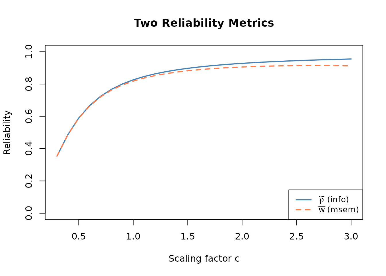

Two-panel plot showing reliability metric curves and their Jensen gap across scaling factors.

Jensen’s gap between the two reliability metrics across scaling factors.


# Panel 2: The gap
plot(results$c, results$gap, type = "l", col = "darkred", lwd = 2,
     xlab = "Scaling factor c", ylab = expression(tilde(rho) - bar(w)),
     main = "Jensen's Gap")
abline(h = 0, lty = 3, col = "gray50")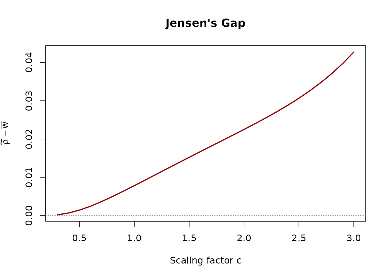

Jensen’s gap between the two reliability metrics across scaling factors.

In this example, the gap is largest at intermediate c values where information varies most across the ability continuum, and shrinks toward zero for very small c where both metrics approach zero. At very large c, the behavior depends on item-location coverage and the empirical grid: logistic saturation can concentrate information into narrow neighborhoods of the item difficulties rather than making information uniformly high.

Scale Ordering Corollary

Corollary 1 (Scale Ordering on a Monotone Branch). Let c^*_{\tilde{\rho}} and c^*_{\bar{w}} denote calibrated scaling factors for the same target \rho^* under the average-information and MSEM metrics, respectively. On a calibration interval where both metrics are continuous and \bar{w}(c) has a unique strictly increasing root for \rho^*, then:

c^*_{\bar{w}} \geq c^*_{\tilde{\rho}} \qquad \text{(9)}

Proof sketch. If \tilde{\rho}(c^*_{\tilde{\rho}}) = \rho^*, then \bar{w}(c^*_{\tilde{\rho}}) \leq \tilde{\rho}(c^*_{\tilde{\rho}}) = \rho^* by Theorem 1. On a branch where \bar{w}(c) is continuous and strictly increasing through the target, reaching \rho^* therefore requires a weakly larger scale. Without this local monotonicity and unique-root condition, Jensen’s inequality gives the pointwise comparison \bar{w}(c) \leq \tilde{\rho}(c) but does not by itself guarantee a global ordering of roots, because \bar{w}(c) can be non-monotone. \square

This ordering is demonstrated numerically below.

# Calibrate the info metric with EQC
eqc_info <- eqc_calibrate(
  target_rho = 0.80, n_items = 25, model = "rasch",
  item_source = "parametric", reliability_metric = "info",
  M = 5000L, seed = 42
)

# Calibrate MSEM on the same realized item form. Because an EQC object carries
# an info-metric contract, pass only its numeric scale as the initializer.
fixed_rasch <- list(
  custom_params = list(
    beta = eqc_info$beta_vec,
    lambda = eqc_info$lambda_base
  ),
  center_difficulties = FALSE
)
sac_msem <- sac_calibrate(
  target_rho = 0.80, n_items = 25, model = "rasch",
  item_source = "custom", item_params = fixed_rasch,
  reliability_metric = "msem", resample_items = FALSE,
  c_init = eqc_info$c_star, n_iter = 200L, M_per_iter = 500L,
  M_pre = 5000L, seed = 42, verbose = FALSE,
  preflight_controls = list(M = 500L),
  evaluation_controls = list(n_forms = 3L, M = 1000L)
)

cat(sprintf("Target rho* = 0.80\n"))
#> Target rho* = 0.80
cat(sprintf("  c* (info metric): %.4f\n", eqc_info$c_star))
#>   c* (info metric): 0.8995
cat(sprintf("  c* (msem metric): %.4f\n", sac_msem$c_star))
#>   c* (msem metric): 0.9179
cat(sprintf("  c*_msem >= c*_info: %s\n",
            sac_msem$c_star >= eqc_info$c_star - 1e-6))
#>   c*_msem >= c*_info: TRUE

Global Discrimination Scaling

The central design variable in IRTsimrel is the global discrimination scaling factor c > 0.

The Scaling Model

Definition 6 (Global Discrimination Scaling). Given baseline item discriminations \boldsymbol{\lambda}^{(0)} = (\lambda_1^{(0)}, \ldots, \lambda_I^{(0)}) generated from an item parameter distribution H, the scaled discriminations are:

\lambda_i(c) = c \cdot \lambda_i^{(0)}, \quad i = 1, \ldots, I \qquad \text{(10)}

This scaling has several desirable properties:

Separation of structure and informativeness: Changing c modifies test information without altering the relative difficulty or discrimination structure among items.
Dimensionality reduction: The multi-dimensional item parameter space is collapsed to a single scalar control variable c.
Smooth dependence on a finite design: For fixed finite theta nodes and a valid item bank, both empirical coefficients are smooth functions of c for c > 0. Extending differentiability through a population expectation requires the corresponding domination and integrability conditions; these fail for some heavy-tail MSEM settings.

For a 3PL bank, \boldsymbol{\beta} and \boldsymbol{g} remain fixed while only \boldsymbol{\lambda}^{(0)} is multiplied. Thus the calibration scale c is not an item guessing parameter. Internally the model is normalized to the D=1 logistic convention.

Rasch/2PL monotonicity on regular calibration intervals

Proposition 1 (Monotonicity; cf. Proposition A.1, Lee 2026). Under the Rasch/2PL regularity and coverage conditions stated in the manuscript, the average-information reliability \tilde{\rho}(c) is strictly monotonically increasing on the population calibration interval.

Branch-qualified caveat. This is a population/practical-interval statement, not a global shape guarantee. A finite empirical quadrature curve can have several extrema and several target crossings, even for a 2PL bank; 3PL tail attenuation makes global monotonicity still less defensible. Version 0.3.0 therefore scans the complete user-supplied interval on \log(c), refines detected features, enumerates roots, and selects a branch explicitly. The default root_policy = "lowest_increasing" chooses the smallest detected crossing with positive local slope. The configured scan has a finite resolution, so its topology diagnostics are evidence within that resolution, not a proof that an arbitrarily narrow unobserved feature cannot exist.

Proof sketch. A full proof is given in Proposition A.1 of the manuscript. From Eq. (5), by the chain rule and the fact that h(x) = x/(x+1) is strictly increasing for x > 0, it suffices to establish that the population average information \bar{\mathcal{J}}(c) = \mathbb{E}_G[\mathcal{J}(\theta; c)] increases on the regular target interval.

For a Rasch/2PL item, direct differentiation gives

\frac{\partial \mathcal{J}_i(\theta; c)}{\partial c} = 2c\, (\lambda_i^{(0)})^2\, p_i(1-p_i) + c^2\, (\lambda_i^{(0)})^2\, p_i(1-p_i)(1-2p_i) \cdot \lambda_i^{(0)}(\theta - \beta_i)

The sign of the pointwise derivative need not be positive at every \theta; the population result is an integrated statement. The manuscript’s argument uses the representation \bar{\mathcal{J}}(c) = c^2 \sum_i (\lambda_i^{(0)})^2 \mathbb{E}[p_i(\theta;c)(1-p_i(\theta;c))] with fixed item locations, positive baseline discriminations, and regular population mass around the item locations. Under these conditions, increasing c raises the population-average information over the stated calibration interval, and therefore increases \tilde{\rho}(c). Outside that interval the package relies on the observed root topology rather than extending the theorem globally. \square

This proof representation is not the derivative of the 3PL information function when g_i>0. Version 0.3.0 makes no corresponding global 3PL monotonicity claim; 3PL calibration uses the same numerical topology scan and requires the selected root’s local direction to be admissible.

Existence and Uniqueness

Corollary 2 (Existence and Uniqueness; cf. Corollary 2.1, Lee 2026). Under the same regularity conditions, consider a practical calibration interval [c_L, c_U] on which \tilde{\rho}(c) is continuous and strictly increasing. For any target \rho^* \in (\rho_L, \rho_U) where

\rho_L = \tilde{\rho}(c_L) \quad\text{and}\quad \rho_U = \tilde{\rho}(c_U),

there exists a unique c^* \in (c_L, c_U) satisfying \tilde{\rho}(c^*) = \rho^*.

Proof. Since \tilde{\rho} is continuous (composition of continuous functions) and strictly increasing on the interval (Proposition 1), existence and uniqueness follow from the intermediate value theorem and strict monotonicity. In the idealized population limit with adequate difficulty coverage, expanding the interval can approach the familiar range from near-zero to near-one reliability; the package nevertheless reports feasibility for the user-supplied finite interval. \square

Non-Monotonicity of MSEM Reliability

Proposition 2 (Non-Monotonicity of MSEM; cf. Proposition A.5, Lee 2026). The MSEM-based reliability \bar{w}(c) is not necessarily monotone in c over the entire positive real line. In particular, for sufficiently large c, \bar{w}(c) can decrease.

Intuition. Under Rasch/2PL, as c \to \infty, for most \theta values far from any \beta_i, the item response probabilities p_i(\theta) approach 0 or 1, causing item information \mathcal{J}_i(\theta)=\lambda_i^2p_i(1-p_i)\to0. Under 3PL the low tail probability approaches g_i, but its derivative and information still vanish; positive guessing makes that low-tail information attenuation faster. Only \theta values very close to some \beta_i retain high information. The harmonic mean (used in \bar{w}) is dominated by the low-information regions, causing \mathbb{E}[1/\mathcal{J}] to grow and \bar{w} to decrease.

The arithmetic mean (used in \tilde{\rho}) is less sensitive to these low- information tails, but that fact alone does not imply global monotonicity on a finite grid.

This is why the c_bounds parameter matters in practice, especially when using the "msem" metric.

Tail integrability is part of the estimand

For any finite logistic item bank, 1/\mathcal{J}(\theta;c) grows at least exponentially in a sufficiently remote tail. A Student-t population has only polynomial tail decay, so \mathbb{E}_G[1/\mathcal{J}(\theta;c)]=\infty for every c>0. Positive 3PL guessing makes the low-ability divergence faster. It follows that population MSEM reliability is zero/undefined for the built-in heavy_tail population; a finite Monte Carlo prefix is an empirical truncated approximation and must not be reported as that population estimand. sac_calibrate() rejects the combination latent_shape = "heavy_tail" and reliability_metric = "msem" before iteration. Average-information reliability remains a separate, potentially finite target.

# Demonstrate non-monotonicity with a heavy-tailed distribution.
# Non-monotonicity is most prominent with heavy tails because extreme
# theta values far from any beta_i have near-zero information, and
# the harmonic mean (used in rho_bar) is dominated by these regions.
theta_nm <- sim_latentG(5000, shape = "heavy_tail", shape_params = list(df = 3))$theta

# Use 10 items with concentrated difficulties for a more visible effect
items_nm <- sim_item_params(10, model = "rasch", source = "parametric")
beta_nm  <- items_nm$data$beta
lambda_nm <- rep(1, 10)

c_wide <- seq(0.1, 15, length.out = 100)
rho_t <- rho_b <- numeric(length(c_wide))

for (j in seq_along(c_wide)) {
  both <- compute_rho_both(c_wide[j], theta_nm, beta_nm, lambda_nm)
  rho_t[j] <- both$rho_tilde
  rho_b[j] <- both$rho_bar
}

oldpar <- par(mar = c(4.5, 4.5, 3, 1))
on.exit(par(oldpar))

plot(c_wide, rho_t, type = "l", col = "steelblue", lwd = 2,
     xlab = "Scaling factor c", ylab = "Reliability",
     main = "Monotonicity Comparison (Heavy-Tailed Latent, df = 3)",
     ylim = c(0, 1))
lines(c_wide, rho_b, col = "coral", lwd = 2, lty = 2)

# Mark the maximum of rho_bar
idx_max <- which.max(rho_b)
points(c_wide[idx_max], rho_b[idx_max], pch = 19, col = "coral", cex = 1.5)

legend("right",
       legend = c(expression(tilde(rho) ~ "(empirical info curve)"),
                  expression(bar(w) ~ "(non-monotone at extreme c)")),
       col = c("steelblue", "coral"), lty = c(1, 2), lwd = 2, cex = 0.85)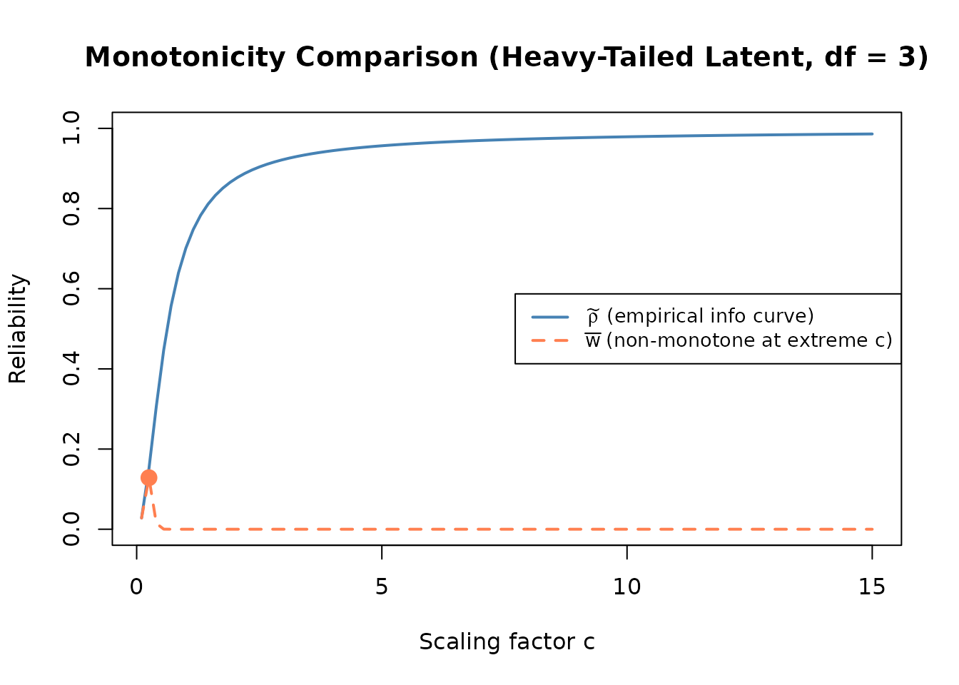

Line plot showing MSEM reliability becoming non-monotone at extreme scaling values under a heavy-tailed latent distribution.

Non-monotonicity of the MSEM metric at extreme scaling factors (heavy-tailed latent distribution, df = 3).


cat(sprintf("rho_bar maximum at c = %.2f with value %.4f\n",
            c_wide[idx_max], rho_b[idx_max]))
#> rho_bar maximum at c = 0.25 with value 0.1285
cat(sprintf("rho_bar at c = %.1f: %.4f (decreasing)\n",
            max(c_wide), rho_b[length(c_wide)]))
#> rho_bar at c = 15.0: 0.0000 (decreasing)

Achievable Reliability Bounds

Not every target reliability is achievable for a given test configuration. The feasible range depends on the number of items, the item parameter distribution, and the latent trait distribution.

A 2PL Upper Bound from the Logistic Kernel

Proposition 3 (Information Upper Bound). Under the 2PL model, the maximum item information is:

\sup_{\theta}\, \mathcal{J}_i(\theta) = \frac{\lambda_i^2}{4} \qquad \text{(11)}

achieved when \theta = \beta_i (i.e., p_i = 1/2). Therefore, test information satisfies:

\sup_{\theta}\, \mathcal{J}(\theta; c) \;\leq\; \frac{c^2}{4} \sum_{i=1}^{I} (\lambda_i^{(0)})^2 \qquad \text{(12)}

Equality in (12) requires the itemwise maxima to occur at the same ability value—in particular, all relevant difficulties must coincide. For the Rasch model with \lambda_i^{(0)} = 1, the right-hand upper bound simplifies to c^2 I / 4; it is not generally the attained maximum when difficulties vary.

This 1/4 bound is a Rasch/2PL result. With 3PL guessing, the information maximum is shifted and reduced, so IRTsimrel evaluates the realized 3PL bank directly instead of substituting the 2PL bound.

Proof. The function p(1-p) on [0,1] has a unique maximum of 1/4 at p = 1/2. Under the 2PL model, p_i(\theta) = 1/2 when \theta = \beta_i. Summing the itemwise bounds gives (12), while simultaneous equality requires a common maximizing \theta. \square

A 2PL analytic feasibility bound

For Rasch/2PL, the average test information is bounded above by the maximum:

\bar{\mathcal{J}}(c) = \mathbb{E}_G\!\left[\sum_{i=1}^{I} \lambda_i(c)^2\, p_i(1-p_i)\right] \leq \frac{c^2}{4} \sum_{i=1}^{I} (\lambda_i^{(0)})^2

Therefore an analytic upper bound on average-information reliability for a given c is:

\tilde{\rho}_{\max}(c) = \frac{\sigma^2_\theta \cdot (c^2/4) \sum_i (\lambda_i^{(0)})^2} {\sigma^2_\theta \cdot (c^2/4) \sum_i (\lambda_i^{(0)})^2 + 1}

This upper bound approaches 1 as c\to\infty; that does not imply the actual finite-form reliability curve is monotone or attains 1. For 3PL and for actual feasibility decisions, the package evaluates the realized curve on the configured interval.

Connection to `check_feasibility()`

The check_feasibility() function uses a shared adaptive log-scale topology scan. The achievable range combines boundaries with polished detected extrema; the result includes root counts, target status, best-achievable points, and the scanner diagnostics. Endpoint values alone are retained as legacy diagnostics and are not assumed to determine the global range.

# Check feasibility for a 25-item Rasch test
feas <- check_feasibility(
  n_items = 25, model = "rasch",
  latent_shape = "normal",
  item_source = "parametric",
  target_rho = 0.80,
  c_bounds = c(0.1, 10),
  M = 5000L, seed = 42
)
#> 
#> =======================================================
#>   Feasibility Check: Achievable Reliability Range
#> =======================================================
#> 
#>   Number of items  : 25
#>   Model            : RASCH
#>   Latent shape     : normal
#>   Latent variance  : 1.0099
#>   c range          : [0.10, 10.00]
#>   Monte Carlo M    : 5000
#> 
#> Achievable Reliability Ranges:
#>   rho_tilde (info) : [0.0591, 0.9872]
#>   rho_bar   (msem) : [0.0002, 0.9146]
#> 
#> Target rho*        : 0.8000
#>   info status      : feasible
#>   msem status      : feasible
#> 
#> Note: rho_tilde >= rho_bar on the same information grid (Jensen's inequality).
#>   rho_tilde range screens EQC targets; root policy must still admit a root.
#>   rho_bar range screens SAC targets; stable interior-branch preflight is also required.

# Test which targets are feasible
targets <- c(0.50, 0.70, 0.80, 0.90, 0.95)
for (rho in targets) {
  feas_rho <- check_feasibility(
    n_items = 25, model = "rasch",
    latent_shape = "normal",
    item_source = "parametric",
    target_rho = rho,
    c_bounds = c(0.1, 10),
    M = 5000L, seed = 42,
    verbose = FALSE
  )
  cat(sprintf("  rho* = %.2f: info %s, msem %s\n",
              rho,
              feas_rho$target_status_info,
              feas_rho$target_status_msem))
}
#>   rho* = 0.50: info feasible, msem feasible
#>   rho* = 0.70: info feasible, msem feasible
#>   rho* = 0.80: info feasible, msem feasible
#>   rho* = 0.90: info feasible, msem feasible
#>   rho* = 0.95: info feasible, msem above_upper

Reliability Curves

The rho_curve() function visualizes how reliability changes with the scaling factor.

curve_data <- rho_curve(
  c_values = seq(0.1, 5, length.out = 60),
  n_items = 25, model = "rasch",
  latent_shape = "normal",
  item_source = "parametric",
  metric = "both",
  M = 5000L, seed = 42,
  plot = TRUE
)

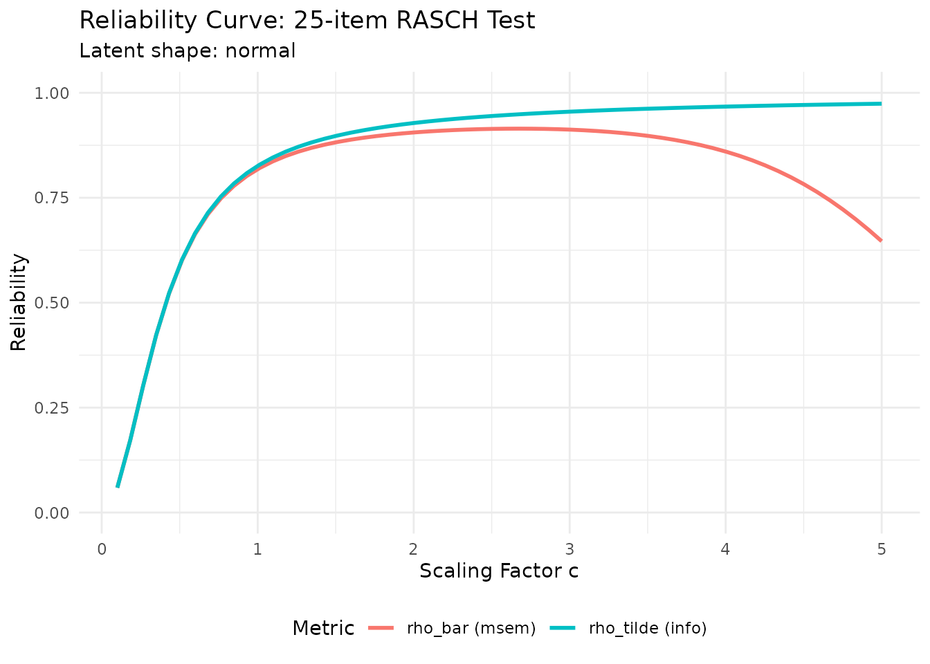
Reliability curve for a 25-item Rasch test under a normal latent distribution.

EQC Theory: Deterministic Root-Finding

The Empirical Quadrature Calibration (EQC) algorithm solves the inverse reliability problem using deterministic root-finding on an empirical reliability function. Full algorithmic details are in vignette("algorithm-eqc"); here we state the main theoretical results.

Algorithm Sketch

EQC proceeds in three steps:

Quadrature sampling: Draw \{\theta_m\}_{m=1}^M \sim G and item parameters \{(\beta_i, \lambda_i^{(0)})\}_{i=1}^I \sim H once.
Empirical reliability function: For any c > 0, define: \hat{\tilde{\rho}}_M(c) = \tilde{\rho}\bigl(c;\, \{\theta_m\},\, \boldsymbol{\beta},\, \boldsymbol{\lambda}(c)\bigr) \qquad \text{(13)}
Topology and root selection: Evaluate an adaptive grid on \log(c), refine detected extrema and target crossings, polish each sign-changing bracket with Brent’s method, and select an admissible root according to root_policy. The default is the lowest increasing crossing.

The scanner never expands c_bounds. Its root table distinguishes crossings, tangencies, boundaries, and plateaus and records local slope direction. If a target is outside the detected range, EQC returns the best-achievable point with an explicit infeasibility status; if topology is unresolved or a feasible target has no root admissible under the requested policy, it raises a classed error rather than silently choosing another branch.

Consistency

Theorem 2 (Branch-conditional consistency of EQC; cf. Theorem A.1, Lee 2026). Let c^* be an isolated population root on a specified increasing branch, and let \hat{c}^*_M be the corresponding EQC root with quadrature size M. Under uniform convergence and local root-separation conditions:

\hat{c}^*_M \xrightarrow{\text{a.s.}} c^* \quad \text{as } M \to \infty \qquad \text{(14)}

Proof sketch. The empirical reliability \hat{\tilde{\rho}}_M(c) converges uniformly to \tilde{\rho}(c) over the compact interval [c_{\min}, c_{\max}] by the Uniform Law of Large Numbers (ULLN). Since \tilde{\rho}(c) is continuous and strictly monotone on that population branch, and the selected root is isolated, uniform convergence of the objective implies convergence of the matching empirical root. This is not a theorem that the whole configured interval has a unique root. \square

Asymptotic Normality

Theorem 3 (Asymptotic Normality of EQC; cf. Theorem A.2, Lee 2026). Under regularity conditions, the EQC estimator satisfies:

\sqrt{M}\,\bigl(\hat{c}^*_M - c^*\bigr) \xrightarrow{d} N\!\left(0,\, \frac{\sigma^2_g}{g'(c^*)^2}\right) \qquad \text{(15)}

where g(c) = \rho(c) - \rho^*, g'(c^*) is the derivative of the reliability function at the solution, and \sigma^2_g is the asymptotic variance of the empirical estimating-function value \hat{\rho}_M(c^*)-\rho^* (the root residual), not a variance of the derivative g'(c^*).

Proof sketch. Apply the delta method to the implicit function \hat{c}^*_M = g^{-1}_M(\rho^*). The Central Limit Theorem gives \sqrt{M}(\hat{\rho}_M(c) - \rho(c)) \to_d N(0, \sigma^2_g), and the implicit function theorem (applicable since g'(c^*) \neq 0 by strict monotonicity) yields the result. \square

Monte Carlo Error Bounds

The practical implication of Theorem 3 is:

|\hat{c}^*_M - c^*| = O_p\!\left(\frac{1}{\sqrt{M}}\right) \qquad \text{(16)}

The reliability estimate itself has error:

|\hat{\rho}_M(c) - \rho(c)| = O_p\!\left(\frac{1}{\sqrt{M}}\right)

The constants depend on the latent distribution, item bank, target, and local slope; 1/\sqrt{M} is a rate statement, not a universal numerical error table. Independent holdout evaluation is needed because evaluating the selected root on the same quadrature grid partly verifies the equation by construction.

SAC Theory: Stochastic Approximation

The Stochastic Approximation Calibration (SAC) algorithm provides an independent solution path using the Robbins-Monro framework. Full algorithmic details are in vignette("algorithm-sac").

SAC has two distinct item measures. With resample_items = FALSE, it targets reliability conditional on one fixed item form. With resample_items = TRUE, it targets the mean of form-level reliabilities over the specified item generator; pooling information across forms would define a different estimand and is not used. The final achieved_rho comes from an independent evaluation bank. compare_eqc_sac() reports agreement only when metric, latent measure, model, item scope, and realized/generator design are comparable; otherwise agreement is NA with reasons.

The Stochastic Root-Finding Problem

SAC targets the equation:

g(c) = \mathbb{E}\!\left[\hat{\rho}(c)\right] - \rho^* = 0 \qquad \text{(17)}

At each iteration n, only a noisy observation \hat{\rho}_n(c_n) = \rho^* + g(c_n) + \varepsilon_n is available, where \varepsilon_n is zero-mean Monte Carlo noise.

Before iteration, version 0.3.0 uses common random numbers to scan the configured interval and identify a stable interior increasing branch. For an item-superpopulation target, split banks must select compatible roots and overlapping branch intervals. The Robbins–Monro projection is then narrowed to that branch. Non-finite topology, an infeasible target, a decreasing or boundary-only solution, or unstable splits produce classed preflight errors. Repeated projection hits can instead return a branch_lost non-convergence status. These guards are part of the implemented algorithm, not merely plotting diagnostics.

Robbins-Monro Update

The iterative update rule is:

c_{n+1} = \Pi_{[c_L, c_U]}\!\left[c_n - a_n\,\bigl(\hat{\rho}_n(c_n) - \rho^*\bigr)\right] \qquad \text{(18)}

where \Pi_{[c_L, c_U]} denotes projection onto the constraint set and the step size sequence satisfies the Robbins-Monro conditions:

a_n = \frac{a}{(n + A)^\gamma}, \quad \sum_{n=1}^{\infty} a_n = \infty, \quad \sum_{n=1}^{\infty} a_n^2 < \infty \qquad \text{(19)}

These conditions are satisfied when \gamma \in (1/2, 1].

Polyak-Ruppert Averaging

Rather than using the final iterate c_N, SAC computes the Polyak-Ruppert average over post-burn-in iterates:

\bar{c}_N = \frac{1}{N - B} \sum_{n=B+1}^{N} c_n \qquad \text{(20)}

where B is the burn-in period. Under the standard regular stochastic-approximation conditions used below, this averaging attains the usual root-n rate.

Convergence

Theorem 4 (Branch-conditional SAC Convergence; cf. Theorem A.3, Lee 2026). Suppose the Robbins–Monro step conditions (Eq. 19) hold; c^* is an interior isolated root of the projected selected branch; g is Lipschitz there and satisfies the branch-wide stability condition (c-c^*)g(c)>0 for every c\ne c^* in that projection interval; and the Monte Carlo error is a martingale difference with bounded conditional variance. Then the projected SAC iterates converge almost surely:

c_n \xrightarrow{\text{a.s.}} c^* \quad \text{as } n \to \infty \qquad \text{(21)}

Furthermore, the Polyak-Ruppert average satisfies:

\sqrt{N - B}\,(\bar{c}_N - c^*) \xrightarrow{d} N\!\left(0,\, \frac{\sigma^2_\varepsilon}{g'(c^*)^2}\right) \qquad \text{(22)}

giving root error O_p(n^{-1/2}) under the additional CLT regularity conditions, compared with the typical O_p(n^{-\gamma/2}) last-iterate error for a step sequence of order n^{-\gamma}.

Proof sketch. Almost sure convergence follows from the classical Robbins-Monro theorem (Robbins and Monro, 1951), extended to the projected case by Kushner and Yin (2003). The key conditions are: (i) g(c^*) = 0, (ii) the branch-wide stability condition above together with g'(c^*) > 0 locally, (iii) the step-size conditions in Eq. (19), and (iv) bounded conditional variance \text{Var}(\varepsilon_n \mid c_n) \leq \sigma^2_\varepsilon. Asymptotic normality of the Polyak-Ruppert average follows from Polyak and Juditsky (1992). The theorem is conditional on the selected branch and does not rescue a run whose branch is absent, non-integrable, or lost. A finite configured preflight scan is diagnostic evidence, not a proof of the branch-wide drift assumption. \square

Numerical Demonstrations

Verifying Theoretical Predictions

We use the low-level reliability functions to verify key theoretical properties.

# Common setup for demonstrations
M_demo <- 5000L
theta_demo <- sim_latentG(M_demo, shape = "normal")$theta
items_demo <- sim_item_params(30, model = "rasch", source = "parametric")
beta_demo  <- items_demo$data$beta
lambda_demo <- rep(1, 30)
theta_var_demo <- var(theta_demo)

Verification 1: Reliability increases with c (info metric)

c_test <- c(0.5, 1.0, 1.5, 2.0, 2.5, 3.0)
rho_info <- sapply(c_test, function(cc) {
  compute_rho_tilde(cc, theta_demo, beta_demo, lambda_demo,
                    theta_var = theta_var_demo)
})

cat("Monotonicity check (info metric):\n")
#> Monotonicity check (info metric):
for (j in seq_along(c_test)) {
  cat(sprintf("  c = %.1f: rho_tilde = %.4f", c_test[j], rho_info[j]))
  if (j > 1) {
    cat(sprintf("  (diff = %+.4f)", rho_info[j] - rho_info[j-1]))
  }
  cat("\n")
}
#>   c = 0.5: rho_tilde = 0.6286
#>   c = 1.0: rho_tilde = 0.8456  (diff = +0.2171)
#>   c = 1.5: rho_tilde = 0.9082  (diff = +0.0626)
#>   c = 2.0: rho_tilde = 0.9351  (diff = +0.0269)
#>   c = 2.5: rho_tilde = 0.9498  (diff = +0.0147)
#>   c = 3.0: rho_tilde = 0.9590  (diff = +0.0092)
cat(sprintf("All differences positive: %s\n", all(diff(rho_info) > 0)))
#> All differences positive: TRUE

Verification 2: Jensen’s gap depends on information heterogeneity

Non-standard latent distributions produce larger Jensen’s gaps because information varies more across the ability continuum.

shapes <- c("normal", "bimodal", "heavy_tail", "skew_pos")
shape_pars <- list(
  normal     = list(),
  bimodal    = list(delta = 0.9),
  heavy_tail = list(df = 5),
  skew_pos   = list(k = 4)
)

c_val <- 1.5
cat(sprintf("Jensen's gap at c = %.1f for different latent shapes:\n", c_val))
#> Jensen's gap at c = 1.5 for different latent shapes:

for (sh in shapes) {
  theta_sh <- sim_latentG(M_demo, shape = sh, shape_params = shape_pars[[sh]])$theta
  both_sh <- compute_rho_both(c_val, theta_sh, beta_demo, lambda_demo)
  gap <- both_sh$rho_tilde - both_sh$rho_bar
  cat(sprintf("  %-12s: rho_tilde = %.4f, rho_bar = %.4f, gap = %.4f\n",
              sh, both_sh$rho_tilde, both_sh$rho_bar, gap))
}
#>   normal      : rho_tilde = 0.9113, rho_bar = 0.9011, gap = 0.0102
#>   bimodal     : rho_tilde = 0.9070, rho_bar = 0.9040, gap = 0.0031
#>   heavy_tail  : rho_tilde = 0.9117, rho_bar = 0.8293, gap = 0.0824
#>   skew_pos    : rho_tilde = 0.9122, rho_bar = 0.8862, gap = 0.0260

Verification 3: APC initialization quality

The Analytic Pre-Calibration (APC) formula provides a closed-form starting point. We compare it against the EQC solution.

targets <- c(0.60, 0.70, 0.80, 0.85, 0.90)
cat("APC initialization vs EQC solution (Rasch, 25 items, normal):\n")
#> APC initialization vs EQC solution (Rasch, 25 items, normal):
cat(sprintf("  %-10s %-10s %-10s %-10s\n", "Target", "c_APC", "c_EQC", "Ratio"))
#>   Target     c_APC      c_EQC      Ratio

for (rho_t in targets) {
  c_apc <- compute_apc_init(target_rho = rho_t, n_items = 25)
  eqc_t <- eqc_calibrate(
    target_rho = rho_t, n_items = 25, model = "rasch",
    item_source = "parametric", M = 5000L, seed = 42, verbose = FALSE
  )
  cat(sprintf("  %-10.2f %-10.4f %-10.4f %-10.2f\n",
              rho_t, c_apc, eqc_t$c_star, c_apc / eqc_t$c_star))
}
#>   0.60       0.8129     0.5118     1.59      
#>   0.70       1.0138     0.6548     1.55      
#>   0.80       1.3274     0.8995     1.48      
#>   0.85       1.5799     1.1199     1.41      
#>   0.90       1.9911     1.5328     1.30

Verification 4: Effect of test length on achievable reliability

n_items_grid <- c(10, 15, 20, 25, 30, 40, 50)
c_fixed <- 1.0

cat(sprintf("Reliability at c = %.1f for different test lengths:\n", c_fixed))
#> Reliability at c = 1.0 for different test lengths:
for (ni in n_items_grid) {
  items_ni <- sim_item_params(ni, model = "rasch", source = "parametric")
  beta_ni  <- items_ni$data$beta
  lambda_ni <- rep(1, ni)

  both_ni <- compute_rho_both(c_fixed, theta_demo, beta_ni, lambda_ni,
                               theta_var = theta_var_demo)
  cat(sprintf("  I = %2d: rho_tilde = %.4f, rho_bar = %.4f\n",
              ni, both_ni$rho_tilde, both_ni$rho_bar))
}
#>   I = 10: rho_tilde = 0.6514, rho_bar = 0.6406
#>   I = 15: rho_tilde = 0.7213, rho_bar = 0.7158
#>   I = 20: rho_tilde = 0.7797, rho_bar = 0.7738
#>   I = 25: rho_tilde = 0.8165, rho_bar = 0.8112
#>   I = 30: rho_tilde = 0.8510, rho_bar = 0.8442
#>   I = 40: rho_tilde = 0.8768, rho_bar = 0.8730
#>   I = 50: rho_tilde = 0.8995, rho_bar = 0.8961

EQC vs SAC Agreement

eqc_demo <- eqc_calibrate(
  target_rho = 0.80, n_items = 25, model = "rasch",
  item_source = "parametric", reliability_metric = "info",
  M = 5000L, seed = 42, verbose = FALSE
)

sac_demo <- sac_calibrate(
  target_rho = 0.80, n_items = 25, model = "rasch",
  reliability_metric = "info", resample_items = FALSE,
  c_init = eqc_demo, n_iter = 300L, M_per_iter = 1000L,
  seed = 42, verbose = FALSE,
  preflight_controls = list(M = 500L),
  evaluation_controls = list(n_forms = 3L, M = 1000L)
)

cat("EQC vs SAC comparison (target = 0.80, info metric):\n")
#> EQC vs SAC comparison (target = 0.80, info metric):
cat(sprintf("  EQC c*:        %.4f\n", eqc_demo$c_star))
#>   EQC c*:        0.8995
cat(sprintf("  SAC c*:        %.4f\n", sac_demo$c_star))
#>   SAC c*:        0.8981
cat(sprintf("  Abs diff:      %.4f\n", abs(eqc_demo$c_star - sac_demo$c_star)))
#>   Abs diff:      0.0014
cat(sprintf("  Pct diff:      %.2f%%\n",
            100 * abs(eqc_demo$c_star - sac_demo$c_star) / eqc_demo$c_star))
#>   Pct diff:      0.15%

Verification 5: Reliability function under the 2PL model

The 2PL model introduces additional variability through heterogeneous baseline discriminations.

items_2pl <- sim_item_params(25, model = "2pl", source = "parametric")
beta_2pl  <- items_2pl$data$beta
lambda_2pl <- if ("lambda_unscaled" %in% names(items_2pl$data)) {
  items_2pl$data$lambda_unscaled
} else {
  items_2pl$data$lambda
}

cat("2PL baseline discriminations:\n")
#> 2PL baseline discriminations:
cat(sprintf("  Range: [%.3f, %.3f]\n", min(lambda_2pl), max(lambda_2pl)))
#>   Range: [0.411, 2.144]
cat(sprintf("  Mean:  %.3f\n", mean(lambda_2pl)))
#>   Mean:  1.165
cat(sprintf("  SD:    %.3f\n", sd(lambda_2pl)))
#>   SD:    0.383

# Compare Rasch and 2PL reliability at same c
c_compare <- 1.0
both_rasch <- compute_rho_both(c_compare, theta_demo,
                                beta_demo[1:25], rep(1, 25),
                                theta_var = theta_var_demo)
both_2pl <- compute_rho_both(c_compare, theta_demo,
                              beta_2pl, lambda_2pl,
                              theta_var = theta_var_demo)

cat(sprintf("\nReliability comparison at c = %.1f:\n", c_compare))
#> 
#> Reliability comparison at c = 1.0:
cat(sprintf("  Rasch: rho_tilde = %.4f, rho_bar = %.4f, gap = %.4f\n",
            both_rasch$rho_tilde, both_rasch$rho_bar,
            both_rasch$rho_tilde - both_rasch$rho_bar))
#>   Rasch: rho_tilde = 0.8213, rho_bar = 0.8152, gap = 0.0062
cat(sprintf("  2PL:   rho_tilde = %.4f, rho_bar = %.4f, gap = %.4f\n",
            both_2pl$rho_tilde, both_2pl$rho_bar,
            both_2pl$rho_tilde - both_2pl$rho_bar))
#>   2PL:   rho_tilde = 0.8556, rho_bar = 0.8444, gap = 0.0112

Heterogeneous discriminations typically produce a larger Jensen’s gap because the test information varies more across the ability continuum.

The Inverse Design Problem

The theoretical framework above describes the forward problem: given a scaling factor c, compute the reliability \rho(c). The central contribution of the IRTsimrel package is solving the inverse problem.

Problem Statement

Definition 7 (Inverse Reliability Problem). Given a target marginal reliability \rho^* \in (0, 1), find a global discrimination scaling factor c^* > 0 such that:

\rho(c^*) = \rho^* \qquad \text{(23)}

where \rho denotes either \tilde{\rho} (average-information) or \bar{w} (MSEM-based), depending on the chosen metric. In IRTsimrel, EQC solves the branch-qualified \tilde{\rho} inverse problem, while SAC can solve either same-estimand validation problems ("info") or direct MSEM problems ("msem").

Why the Inverse Problem is Difficult

Several factors make this inverse problem non-trivial:

No closed-form solution: The reliability function involves a logistic nonlinearity inside an expectation over G. Even in the simplest Rasch case with normal G, no analytic inversion is possible.
Distribution dependence: The mapping c \mapsto \rho(c) depends on the full distributions G (latent traits) and H (item parameters), not just their moments.
Metric ambiguity: The two reliability definitions yield different c^* values for the same target (Corollary 1).
Practical constraints: The scaling factor must lie within bounds that produce realistic item parameters.
Root and item scope: A finite curve may have several roots, and a fixed-form coefficient is not the same estimand as an average across random item forms. Both must be specified before a scale can be interpreted.

The APC Approximation

The Analytic Pre-Calibration (APC) formula provides a rough initial estimate under Gaussian Rasch assumptions. With \theta \sim N(0,1) and \beta \sim N(0, \sigma^2_\beta), the expected item information involves the logistic-normal convolution constant:

\kappa(\sigma^2) = \int_{-\infty}^{\infty} \frac{e^z}{(1+e^z)^2}\, \phi(z; 0, \sigma^2)\, dz \approx \frac{0.25}{\sqrt{1 + \sigma^2 \pi^2 / 3}} \qquad \text{(24)}

where \sigma^2 = 1 + \sigma^2_\beta. The APC initial value is:

c_{\text{APC}} = \sqrt{\frac{\rho^*}{I \cdot \kappa \cdot (1 - \rho^*)}} \qquad \text{(25)}

This approximation is typically within a factor of 2 of the true c^* and serves as a starting point for the stochastic approximation algorithm (SAC).

Complete Notation Table

The following table summarizes all mathematical notation used in the package and its documentation.

Symbol	Description	Domain
\theta	Latent ability parameter	\mathbb{R}
G	Latent trait distribution	–
\sigma^2_\theta	Variance of \theta under G	(0, \infty)
\beta_i	Difficulty parameter for item i	\mathbb{R}
\lambda_i	Discrimination parameter for item i	(0, \infty)
\lambda_i^{(0)}	Baseline (unscaled) discrimination	(0, \infty)
g_i	3PL lower asymptote (`guessing`)	[0, 1)
c	Global discrimination scaling factor	(0, \infty)
c^*	Calibrated scaling factor	(0, \infty)
I	Number of items	\mathbb{N}
M	Quadrature (Monte Carlo) sample size	\mathbb{N}
\psi(z)	Logistic function 1/(1+e^{-z})	(0, 1)
p_i(\theta)	P(X_i = 1 \mid \theta); ICC	(0, 1)
\mathcal{J}_i(\theta)	Item information function	(0, \infty)
\mathcal{J}(\theta)	Test information function	(0, \infty)
\bar{\mathcal{J}}(c)	Average test information \mathbb{E}_G[\mathcal{J}(\theta;c)]	(0, \infty)
\tilde{\rho}(c)	Average-information reliability	(0, 1)
\bar{w}(c)	MSEM-based reliability	(0, 1)
\rho^*	Target reliability	(0, 1)
\hat{\rho}_M(c)	Empirical reliability (EQC)	(0, 1)
\hat{\rho}_n(c)	Noisy reliability estimate (SAC)	(0, 1)
a_n	Step size at iteration n	(0, \infty)
a	Step size constant (SAC)	(0, \infty)
A	Stabilization constant (SAC)	[0, \infty)
\gamma	Step decay exponent (SAC)	(1/2, 1]
B	Burn-in period (SAC)	\mathbb{N}_0
N	Total number of SAC iterations	\mathbb{N}
\bar{c}_N	Polyak-Ruppert average	(0, \infty)
\kappa	Logistic-normal convolution constant (APC)	(0, 1/4)
H	Item parameter distribution	–
\text{MSEM}	\mathbb{E}[1/\mathcal{J}(\theta;c)]	(0, \infty)

Summary of Theoretical Results

Result	Statement	Implication
Theorem 1	\tilde{\rho}(c) \geq \bar{w}(c) (Jensen)	Info metric is at least as large on the same population/grid basis
Corollary 1	c^_{\bar{w}} \geq c^_{\tilde{\rho}} on a monotone MSEM branch	MSEM metric requires a weakly larger scale when the MSEM root is unique on the selected interval
Proposition 1	\tilde{\rho}(c) is strictly increasing on regular calibration intervals	Existence and uniqueness for bracketed info targets
Corollary 2	Unique c^* exists for \rho^* \in (\rho_L,\rho_U) on such an interval	EQC root-finding is well-defined after feasibility checks
Proposition 2	\bar{w}(c) is not always monotone	`c_bounds` critical for MSEM metric
Proposition 3	\max \mathcal{J}_i = \lambda_i^2/4 for 2PL	2PL-only analytic upper bound
Theorem 2	EQC consistent for an isolated selected branch (\hat{c}^_M \to c^ a.s.)	Precision increases with M under the stated conditions
Theorem 3	EQC asymptotically normal (\sqrt{M} rate)	Quantifiable uncertainty
Theorem 4	SAC converges locally on an admissible selected branch, with PR averaging	Preflight and branch diagnostics are required

References

Lee, J.-H. (2026). Reliability-Targeted Simulation of Item Response Data: Solving the Inverse Design Problem. arXiv:2512.16012v2. https://doi.org/10.48550/arXiv.2512.16012

Robbins, H., & Monro, S. (1951). A stochastic approximation method. The Annals of Mathematical Statistics, 22(3), 400–407.

Polyak, B. T., & Juditsky, A. B. (1992). Acceleration of stochastic approximation by averaging. SIAM Journal on Control and Optimization, 30(4), 838–855.

Kushner, H. J., & Yin, G. G. (2003). Stochastic Approximation and Recursive Algorithms and Applications (2nd ed.). Springer.

Brent, R. P. (1973). Algorithms for Minimization Without Derivatives. Prentice-Hall.

Lord, F. M. (1980). Applications of Item Response Theory to Practical Testing Problems. Erlbaum.

van der Linden, W. J. (Ed.). (2016). Handbook of Item Response Theory (Vols. 1–3). CRC Press.

Birnbaum, A. (1968). Some latent trait models and their use in inferring an examinee’s ability. In F. M. Lord & M. R. Novick (Eds.), Statistical Theories of Mental Test Scores (pp. 395–479). Addison-Wesley.

JoonHo Lee (jlee296@ua.edu)

2026-08-22