Working with Latent Distributions

1. Overview

The sim_latentG() function generates latent abilities (person parameters \theta) for IRT simulation studies. It implements the population model:

\theta_p \sim G

where G is a flexible distribution family that can take many different shapes while maintaining rigorous standardization properties.

Estimated reading time: 20–25 minutes.

This vignette covers:

The pre-standardization principle
Available distribution shapes (12 supported shapes including custom)
Customizing shape parameters
Creating custom mixture distributions
Adding covariate effects
Visualization tools
How latent shape affects achievable reliability

For the complete applied workflow that uses sim_latentG() as part of reliability-targeted simulation, see vignette("applied-guide").

2. The Pre-Standardization Principle

A key design feature of sim_latentG() is pre-standardization: every built-in distribution shape is mathematically constructed to have mean 0 and variance 1 before any scaling is applied.

This ensures that:

Changing the shape does not inadvertently change the scale
The sigma parameter directly controls the residual standard deviation; covariate variation can increase the marginal SD of theta
Comparisons across shapes are meaningful

The generated abilities follow:

\theta_p = \mu + X_p^\top \beta + \sigma \cdot z_p

where z_p \sim G_0 with \mathbb{E}[z] = 0 and \text{Var}[z] = 1.

2.1 Why This Matters

In traditional simulation approaches, changing the latent distribution often changes both the shape and the scale simultaneously. For example, switching from N(0, 1) to \text{Gamma}(4, 1) changes not just the shape but also the variance.

With pre-standardization, you can study the effect of distributional shape on IRT estimation while holding variance constant – a cleaner experimental design.

3. Basic Usage

# Generate 1000 standard normal abilities
sim_normal <- sim_latentG(n = 1000, shape = "normal", seed = 42)

# Examine the result
print(sim_normal)
#> Latent Ability Distribution (G-family)
#> =======================================
#>   Shape     : normal
#>   n         : 1000
#>   Target mu : 0.0000
#>   Target sigma: 1.0000
#> 
#> Sample Moments:
#>   Mean      : -0.0258
#>   SD        : 1.0025
#>   Skewness  : -0.0038
#>   Kurtosis  : 0.1286 (excess)

The output shows:

Target mu/sigma: The requested location and scale
Sample Moments: Empirical mean, SD, skewness, and excess kurtosis

# Verify standardization
cat(sprintf("Sample mean: %.4f (target: 0)\n", mean(sim_normal$theta)))
#> Sample mean: -0.0258 (target: 0)
cat(sprintf("Sample SD:   %.4f (target: 1)\n", sd(sim_normal$theta)))
#> Sample SD:   1.0025 (target: 1)

4. Available Distribution Shapes

sim_latentG() provides 12 supported shapes, including 11 built-in pre-standardized shapes plus the custom mixture option.

4.1 Standard Normal

The baseline case: z \sim N(0, 1)

sim_normal <- sim_latentG(n = 2000, shape = "normal", seed = 1)
plot(sim_normal, show_normal = TRUE)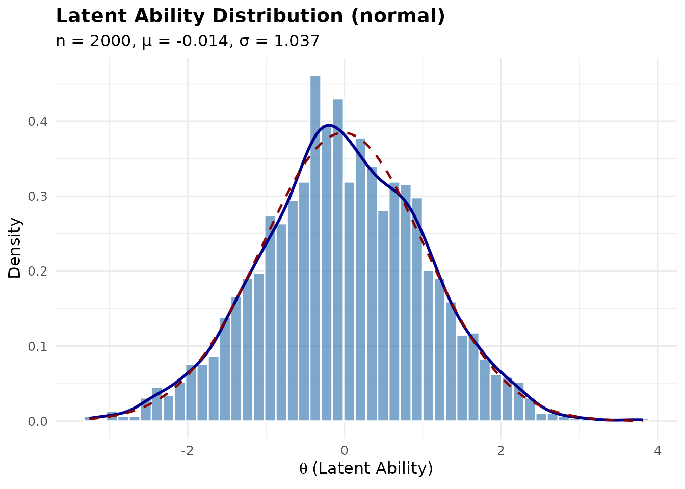

Histogram and density plot of a standard normal latent ability distribution with a normal reference curve.

4.2 Bimodal Distribution

A symmetric two-component Gaussian mixture, useful for representing populations with two distinct subgroups (e.g., native vs. non-native speakers).

Mathematical construction:

z = s \cdot \delta + \epsilon, \quad s \sim \text{Rademacher}(\pm 1), \quad \epsilon \sim N(0, 1 - \delta^2)

The component variance 1 - \delta^2 ensures \text{Var}[z] = \delta^2 + (1 - \delta^2) = 1.

sim_bimodal <- sim_latentG(n = 2000, shape = "bimodal", seed = 1)
plot(sim_bimodal, show_normal = TRUE)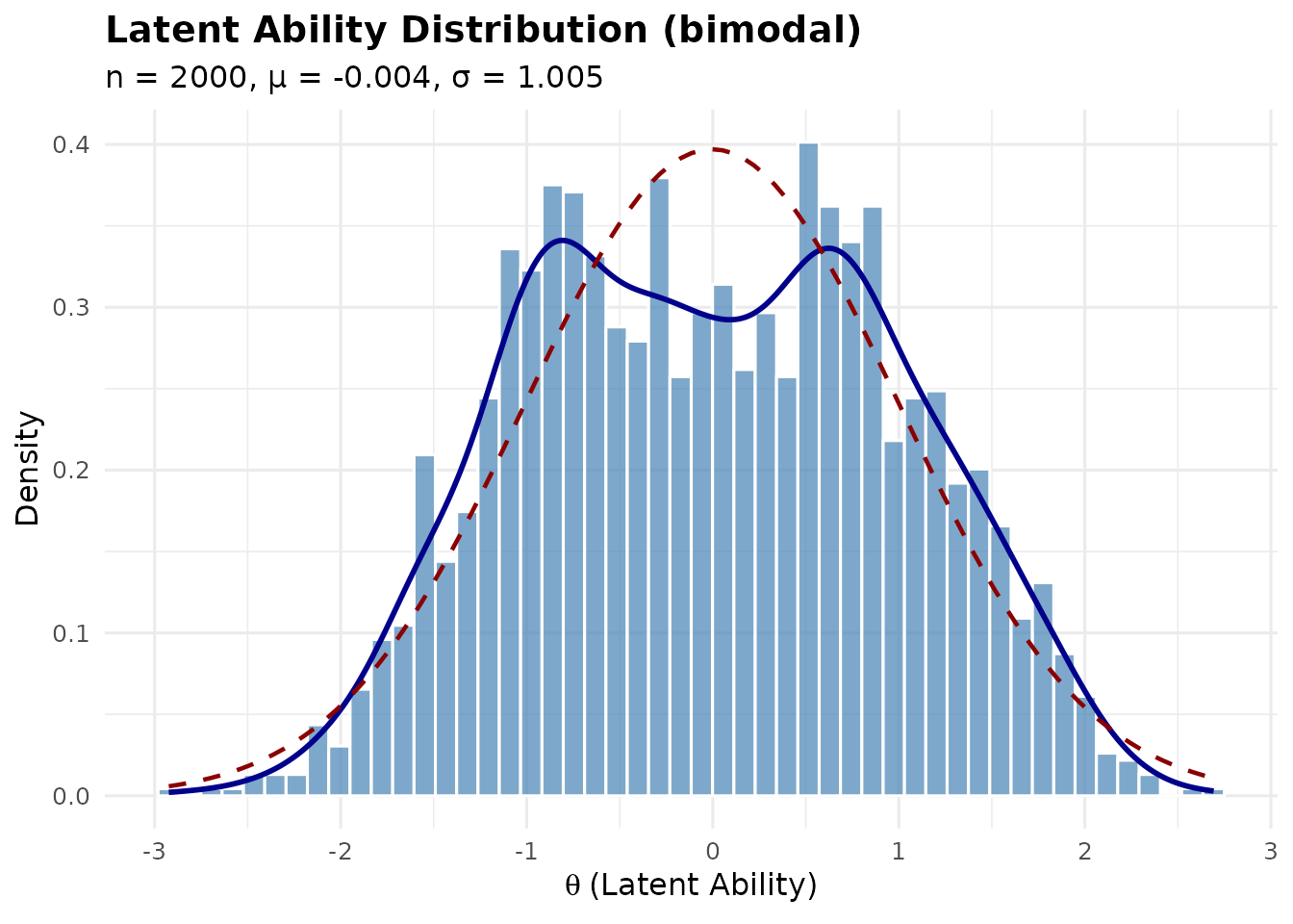

Histogram and density plot of a bimodal latent ability distribution with two symmetric modes.

Customizing mode separation:

The delta parameter controls how far apart the modes are (0 < \delta < 1):

# Wider separation
sim_bimodal_wide <- sim_latentG(
  n = 2000,
  shape = "bimodal",
  shape_params = list(delta = 0.95),
  seed = 1
)
plot(sim_bimodal_wide, show_normal = TRUE)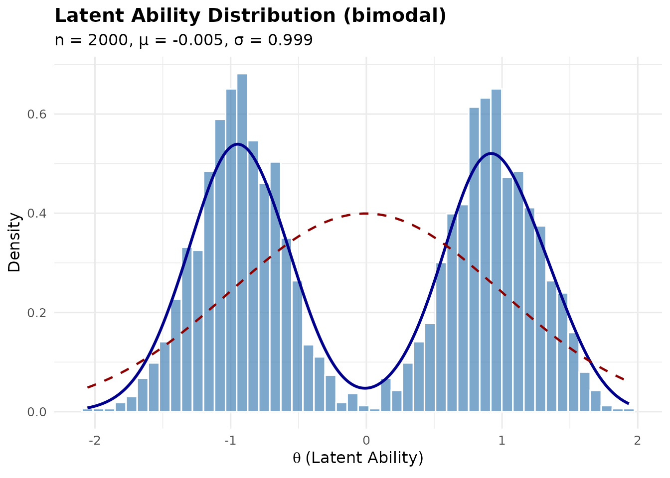

Histogram and density plot of a bimodal latent distribution with wider mode separation.

4.3 Trimodal Distribution

A symmetric three-component mixture with a central peak and two side peaks.

Mathematical construction:

Components at \{-m, 0, +m\} with weights (w_L, w_0, w_R) where w_L = w_R = (1 - w_0)/2.

Component variance: \sigma_c^2 = 1 - (1 - w_0) m^2

sim_trimodal <- sim_latentG(n = 2000, shape = "trimodal", seed = 1)
plot(sim_trimodal, show_normal = TRUE)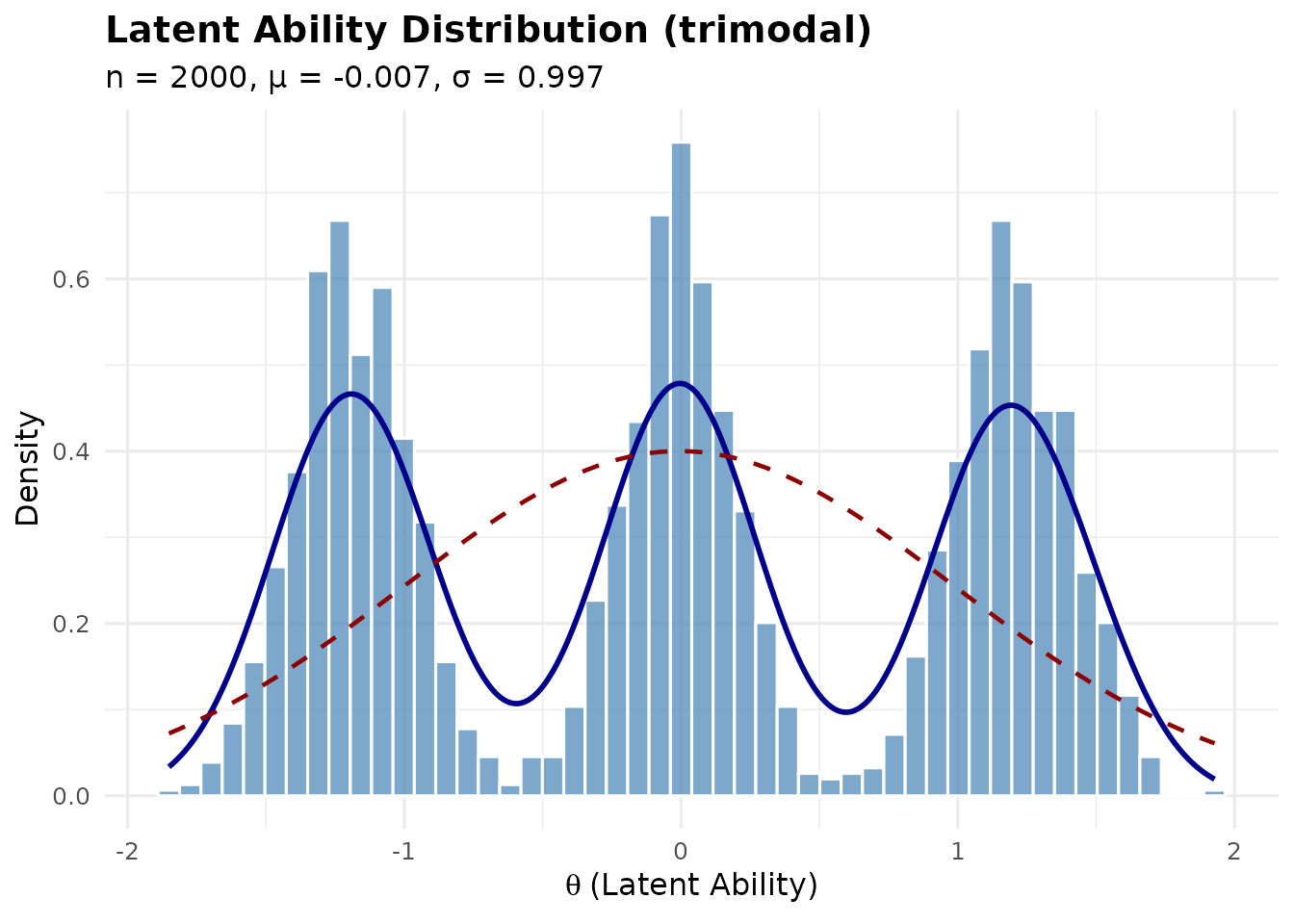

Histogram and density plot of a trimodal latent ability distribution with one central and two side modes.

Customizing:

# Stronger central peak
sim_trimodal_central <- sim_latentG(
  n = 2000,
  shape = "trimodal",
  shape_params = list(
    w0 = 0.5,   # Weight of central component (default: 1/3)
    m = 1.3     # Location of side components (default: 1.2)
  ),
  seed = 1
)
plot(sim_trimodal_central, show_normal = TRUE)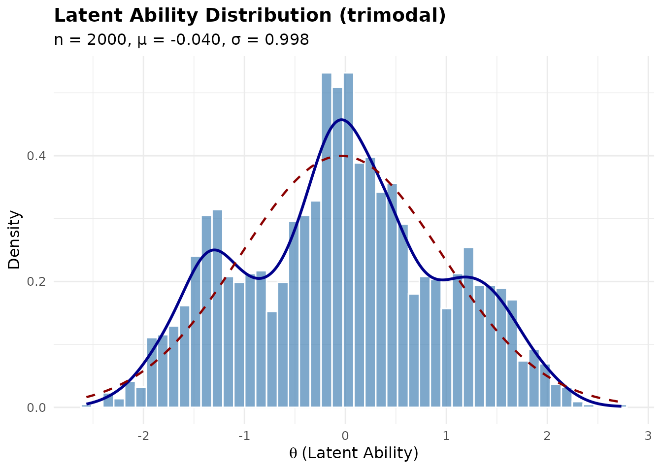

Histogram and density plot of a trimodal latent distribution with a stronger central peak.

4.4 Multimodal (Four Components)

A symmetric four-component mixture with modes at \{-m_2, -m_1, +m_1, +m_2\}.

sim_multi <- sim_latentG(n = 2000, shape = "multimodal", seed = 1)
plot(sim_multi, show_normal = TRUE)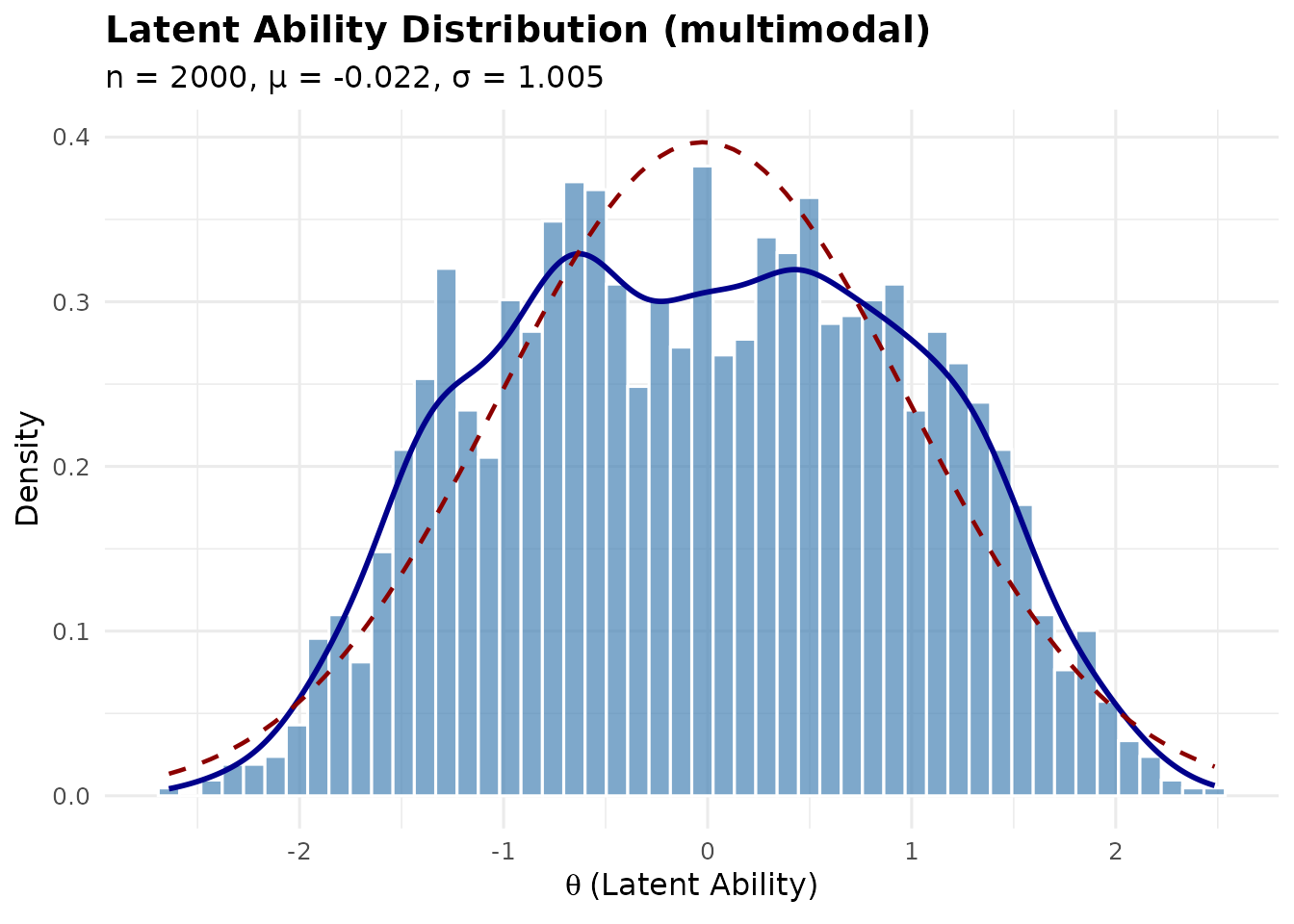

Histogram and density plot of a four-component multimodal latent ability distribution.

4.5 Skewed Distributions

Right-skewed (skew_pos): Based on standardized Gamma distribution:

z = \frac{\Gamma(k, 1) - k}{\sqrt{k}}

This has \mathbb{E}[z] = 0 and \text{Var}[z] = 1 for any k > 0.

sim_skew_pos <- sim_latentG(n = 2000, shape = "skew_pos", seed = 1)
plot(sim_skew_pos, show_normal = TRUE)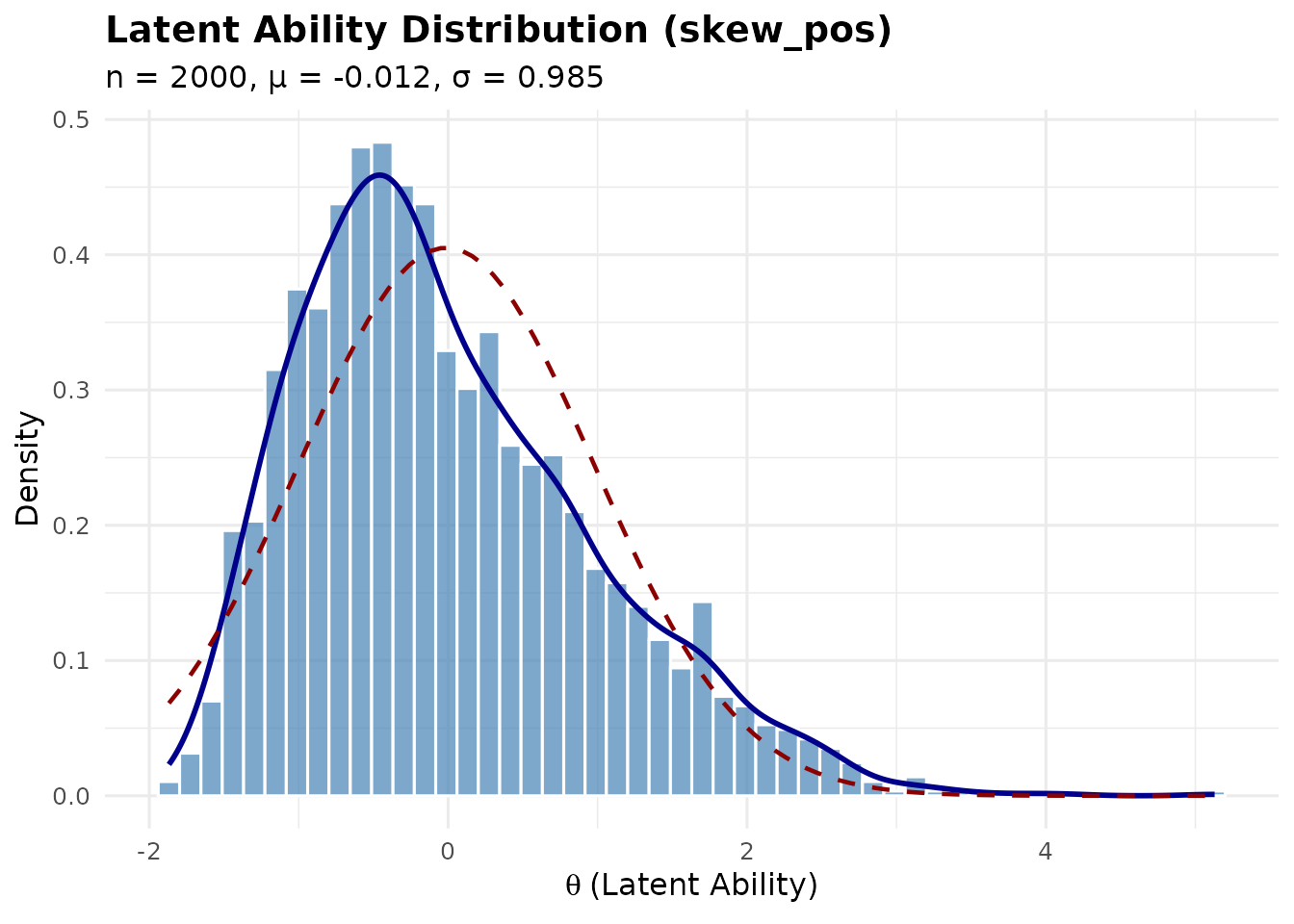

Histogram and density plot of a positively skewed latent ability distribution.

Left-skewed (skew_neg): Simply the negation of the right-skewed distribution.

sim_skew_neg <- sim_latentG(n = 2000, shape = "skew_neg", seed = 1)
plot(sim_skew_neg, show_normal = TRUE)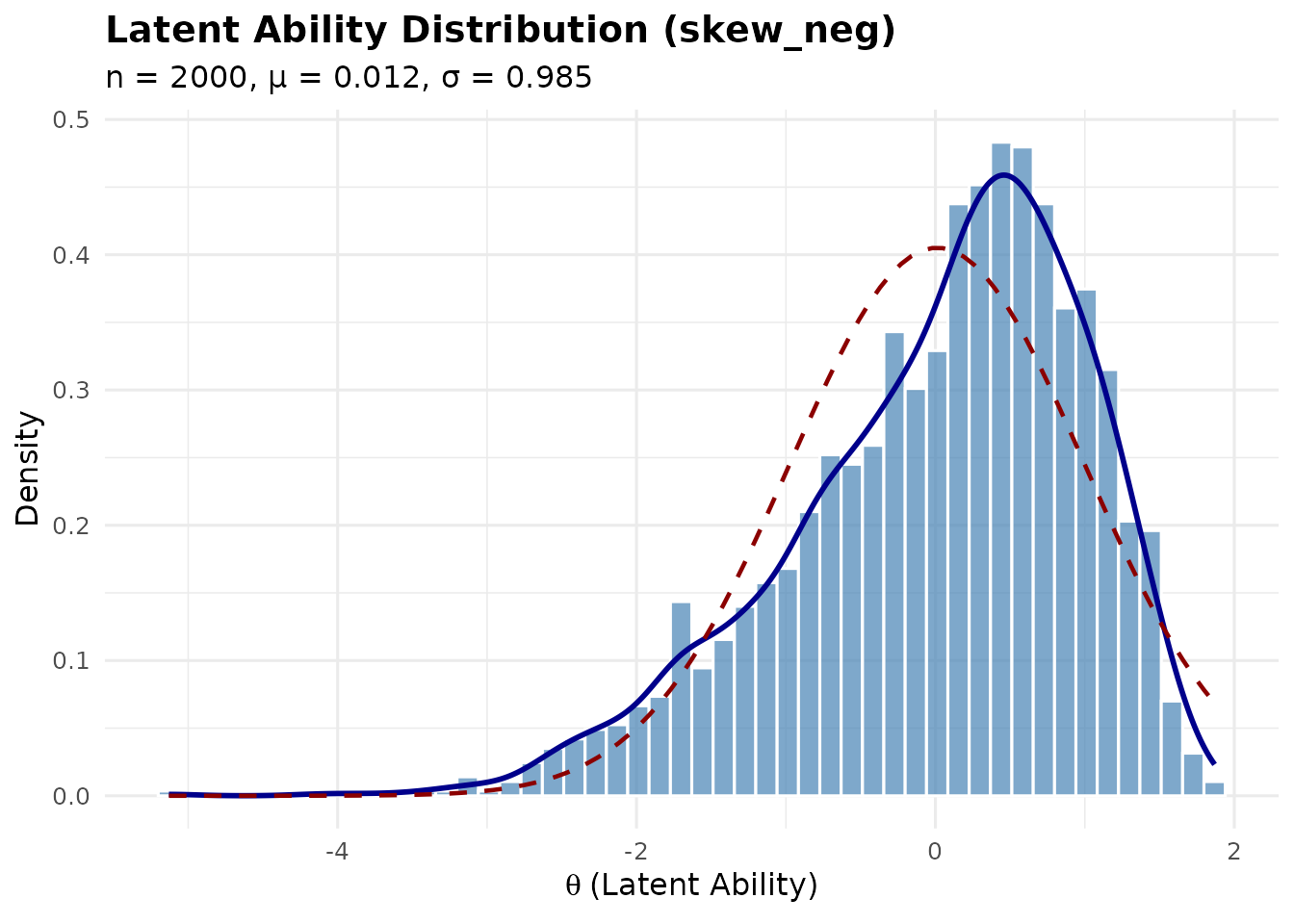

Histogram and density plot of a negatively skewed latent ability distribution.

Controlling skewness magnitude:

The k parameter (Gamma shape) controls skewness – smaller values mean more skewed:

# More extreme skewness (k = 2)
sim_very_skew <- sim_latentG(
  n = 2000,
  shape = "skew_pos",
  shape_params = list(k = 2),
  seed = 1
)

cat(sprintf("Default k=4 skewness: %.3f\n", sim_skew_pos$sample_moments$skewness))
#> Default k=4 skewness: 0.812
cat(sprintf("k=2 skewness:         %.3f\n", sim_very_skew$sample_moments$skewness))
#> k=2 skewness:         1.244

4.6 Heavy-Tailed Distribution

Based on standardized Student-t:

z = \frac{t_\nu}{\sqrt{\nu / (\nu - 2)}}

This has \text{Var}[z] = 1 for \nu > 2.

The built-in Student-t heavy-tail population is suitable for the average-information metric, but not for population MSEM targeting under the reciprocal-information approximation: the expectation of inverse information diverges in the tails. A finite Monte Carlo sample can still return a finite rho_bar, but that number is a sample/grid diagnostic rather than a finite population estimand. SAC rejects this incompatible population-MSEM contract.

sim_heavy <- sim_latentG(n = 2000, shape = "heavy_tail", seed = 1)
plot(sim_heavy, show_normal = TRUE)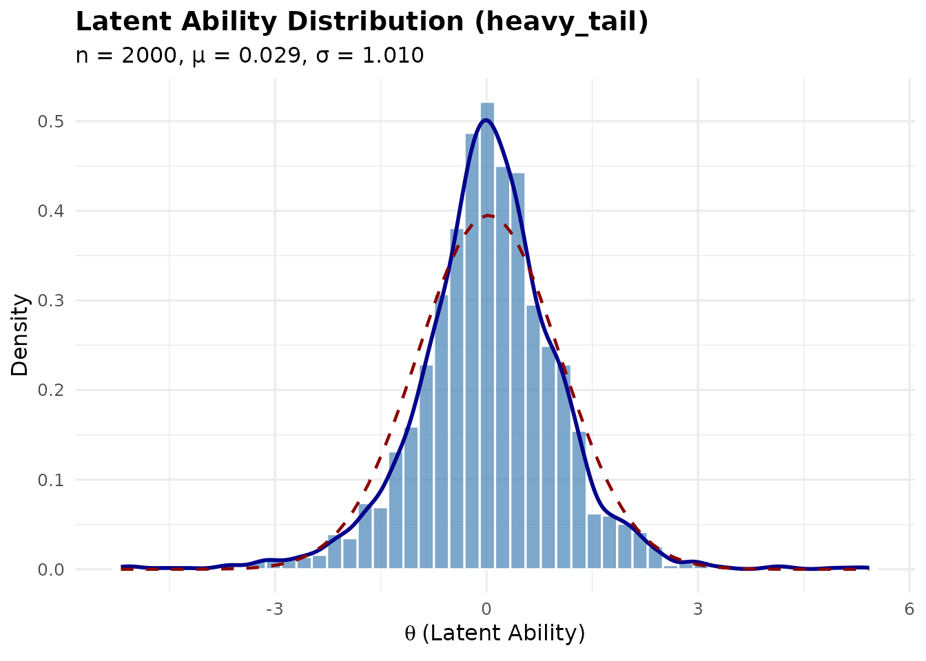

Histogram and density plot of a heavy-tailed latent ability distribution with a normal reference curve.

Controlling tail heaviness:

The df parameter (degrees of freedom) controls tail weight – smaller values mean heavier tails:

# Very heavy tails (df = 3)
sim_very_heavy <- sim_latentG(
  n = 2000,
  shape = "heavy_tail",
  shape_params = list(df = 3),
  seed = 1
)

cat(sprintf("Default df=5 kurtosis: %.3f\n", sim_heavy$sample_moments$kurtosis))
#> Default df=5 kurtosis: 2.924
cat(sprintf("df=3 kurtosis:         %.3f\n", sim_very_heavy$sample_moments$kurtosis))
#> df=3 kurtosis:         7.956

4.7 Light-Tailed (Platykurtic) Distribution

A mixture distribution approximating a platykurtic shape (negative excess kurtosis).

sim_light <- sim_latentG(n = 2000, shape = "light_tail", seed = 1)
plot(sim_light, show_normal = TRUE)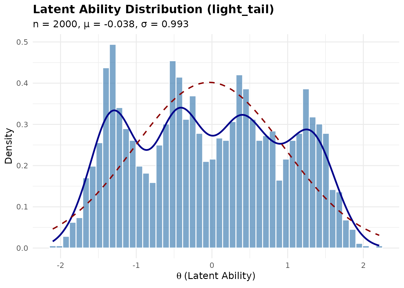

Histogram and density plot of a light-tailed latent ability distribution.

4.8 Uniform Distribution

Uniform on [-\sqrt{3}, +\sqrt{3}], which has mean 0 and variance 1.

sim_uniform <- sim_latentG(n = 2000, shape = "uniform", seed = 1)
plot(sim_uniform, show_normal = TRUE)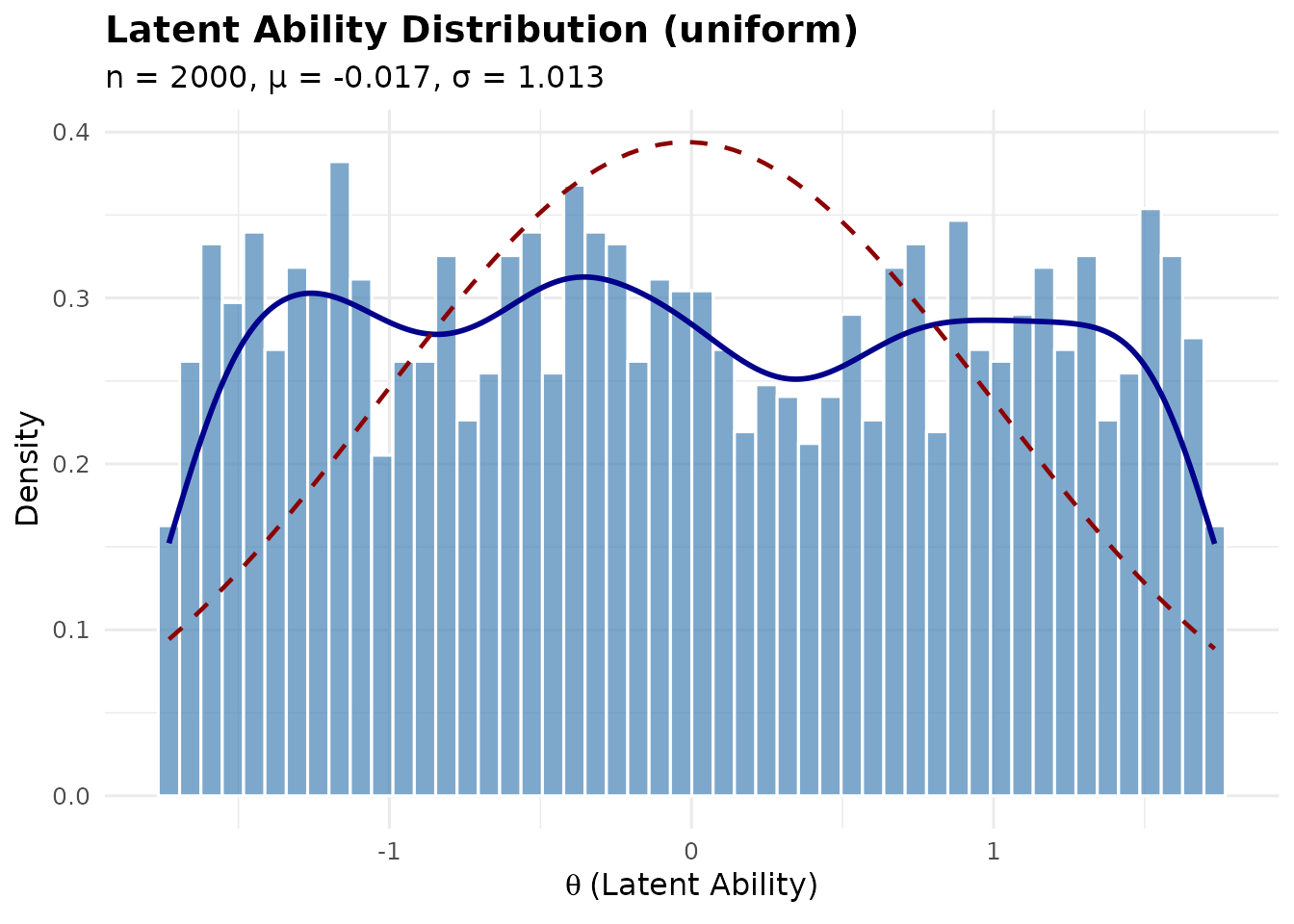

Histogram and density plot of a uniform latent ability distribution.

4.9 Floor and Ceiling Effects

These represent situations where there is a concentration of examinees at one end of the ability distribution.

Floor effect: Heavy component near the lower bound (e.g., many low-ability students in a difficult test)

sim_floor <- sim_latentG(n = 2000, shape = "floor", seed = 1)
plot(sim_floor, show_normal = TRUE)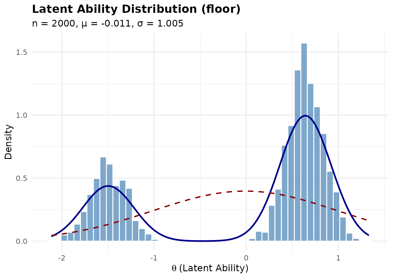

Histogram and density plot of a latent ability distribution with a floor effect.

Ceiling effect: Heavy component near the upper bound (e.g., many high-ability students in an easy test)

sim_ceiling <- sim_latentG(n = 2000, shape = "ceiling", seed = 1)
plot(sim_ceiling, show_normal = TRUE)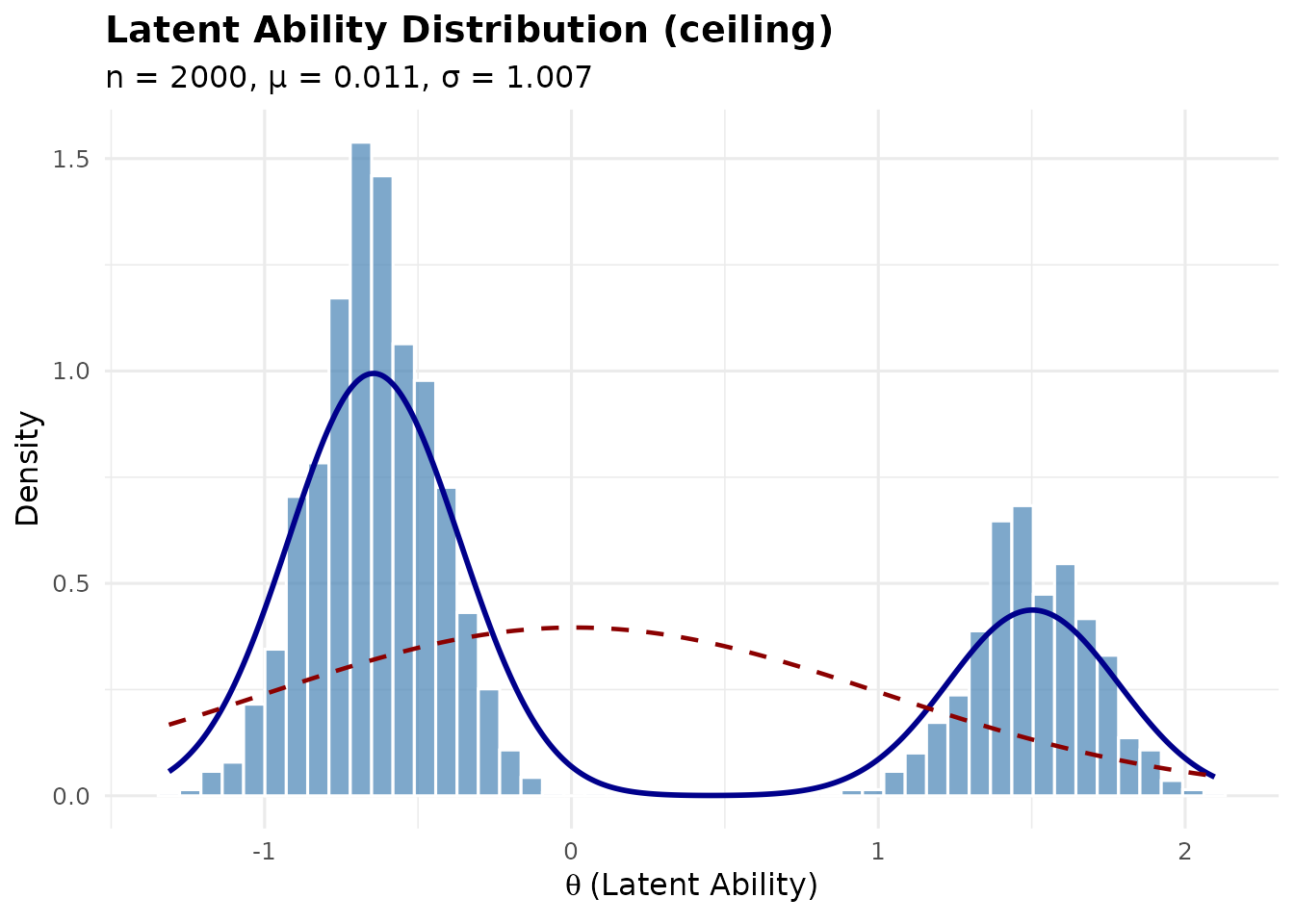

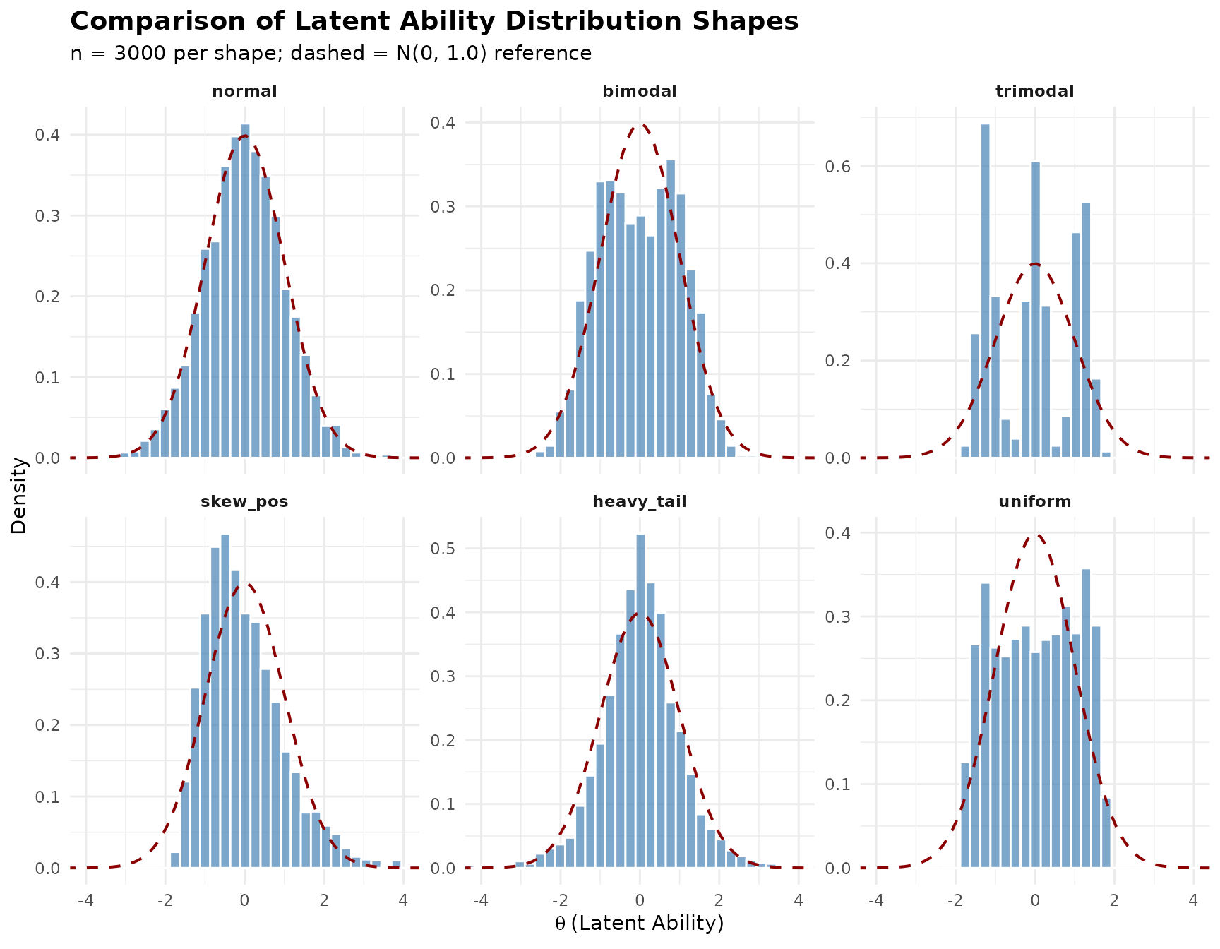
Histogram and density plot of a latent ability distribution with a ceiling effect.

5. Comparing Multiple Shapes

The compare_shapes() function provides a convenient way to visualize multiple distributions side-by-side:

compare_shapes(
  n = 3000,
  shapes = c("normal", "bimodal", "trimodal",
             "skew_pos", "heavy_tail", "uniform"),
  sigma = 1,
  seed = 42
)

Faceted density comparison across all built-in latent distribution shapes.

6. Custom Mixture Distributions

For maximum flexibility, use shape = "custom" with mixture_spec:

# Define a custom 3-component mixture
sim_custom <- sim_latentG(
  n = 2000,
  shape = "custom",
  mixture_spec = list(
    weights = c(0.3, 0.5, 0.2),   # Must sum to 1
    means = c(-1.5, 0, 2),        # Component means
    sds = c(0.5, 0.7, 0.5)        # Component SDs
  ),
  seed = 1
)

plot(sim_custom, show_normal = TRUE)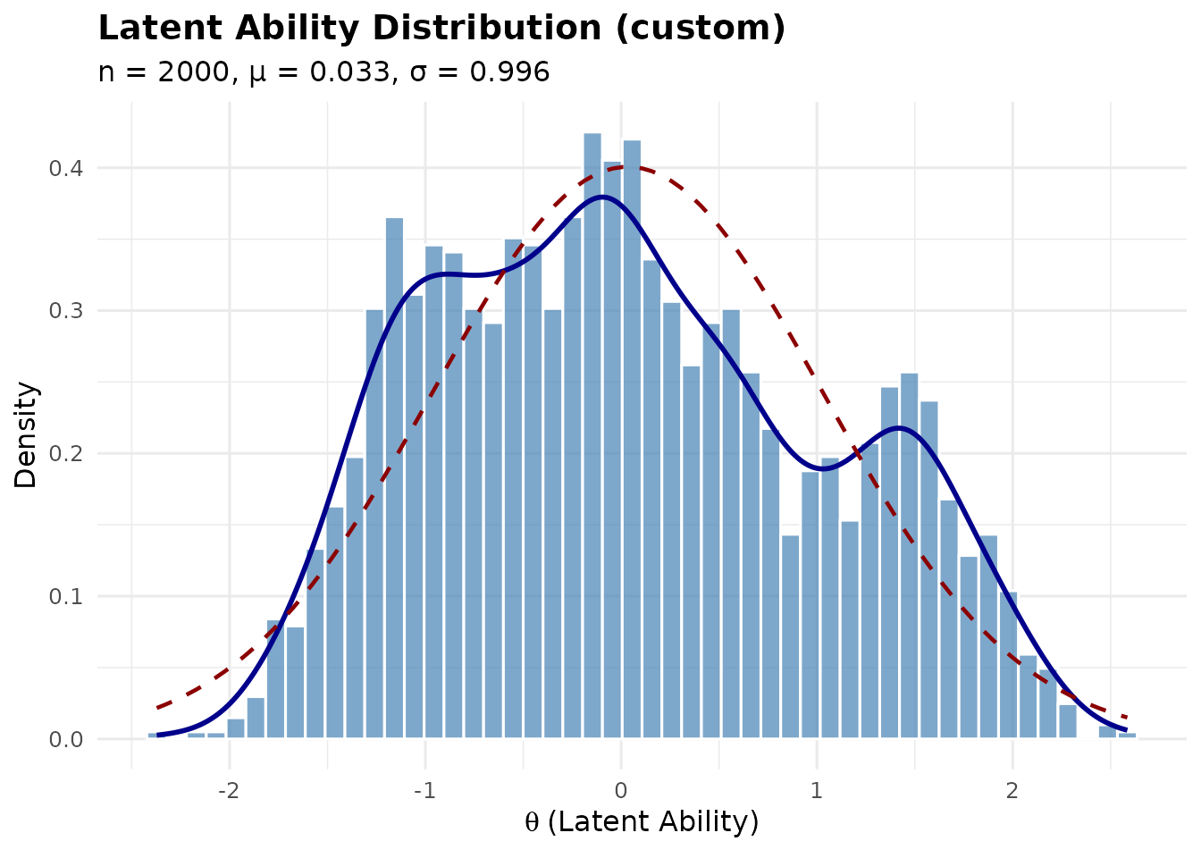

Histogram and density plot of a custom three-component latent mixture distribution.

By default, custom mixtures are automatically post-standardized to have mean 0 and variance 1. To disable this:

# Keep raw mixture parameters
sim_raw <- sim_latentG(
  n = 2000,
  shape = "custom",
  mixture_spec = list(
    weights = c(0.5, 0.5),
    means = c(-1, 1),
    sds = c(0.5, 0.5)
  ),
  standardize_custom = FALSE,
  seed = 1
)

7. Adjusting Location and Scale

The mu and sigma parameters allow you to shift and scale the distribution:

# Generate abilities with mean 100 and SD 15 (like IQ scores)
sim_iq <- sim_latentG(
  n = 1000,
  shape = "normal",
  mu = 100,
  sigma = 15,
  seed = 42
)

summary(sim_iq)
#> Summary: Latent Ability Distribution
#> ====================================
#>   Shape      : normal
#>   n          : 1000
#>   Target     : mu = 100.00, sigma = 15.00
#>   Covariates : No
#> 
#> Sample Statistics:
#>   Mean       : 99.6126
#>   SD         : 15.0378
#>   Median     : 99.8030
#>   Skewness   : -0.0038
#>   Kurtosis   : 0.1286 (excess)
#>   Range      : [49.4239, 152.4296]
#> 
#> Quantiles:
#>     2.5%       5%      25%      50%      75%      95%    97.5% 
#>  69.8816  75.3193  89.8681  99.8030 109.9601 123.0023 128.1655

This works with any shape:

# Bimodal with different scale
sim_bimodal_scaled <- sim_latentG(
  n = 1000,
  shape = "bimodal",
  mu = 0,
  sigma = 1.5,  # Larger spread
  seed = 42
)

cat(sprintf("Sample SD: %.3f (target: 1.5)\n", sd(sim_bimodal_scaled$theta)))
#> Sample SD: 1.481 (target: 1.5)

8. Adding Covariate Effects

You can incorporate person-level covariates that affect ability:

# Create covariate data
n <- 1000
set.seed(42)
group <- rbinom(n, 1, 0.5)           # Binary group indicator
ses <- rnorm(n)                       # Continuous SES measure

# Generate abilities with covariate effects
sim_cov <- sim_latentG(
  n = n,
  shape = "normal",
  xcov = data.frame(group = group, ses = ses),
  beta = c(0.5, 0.3),  # Group effect = 0.5, SES effect = 0.3
  seed = 42
)

# Verify covariate effects
cat("Mean ability by group:\n")
#> Mean ability by group:
cat(sprintf("  Group 0: %.3f\n", mean(sim_cov$theta[group == 0])))
#>   Group 0: -0.084
cat(sprintf("  Group 1: %.3f\n", mean(sim_cov$theta[group == 1])))
#>   Group 1: 0.519
cat(sprintf("  Difference: %.3f (expected: 0.5)\n",
            mean(sim_cov$theta[group == 1]) - mean(sim_cov$theta[group == 0])))
#>   Difference: 0.602 (expected: 0.5)

The full model is:

\theta_p = \mu + X_p^\top \beta + \sigma \cdot z_p

where X_p is the covariate vector for person p.

9. Working with the Output Object

The sim_latentG() function returns a latent_G object containing:

sim <- sim_latentG(n = 100, shape = "bimodal", seed = 1)

# Available components
names(sim)
#> [1] "theta"          "mu"             "sigma"          "eta_cov"       
#> [5] "shape"          "shape_params"   "n"              "sample_moments"
#> [9] "z"

# The theta vector
head(sim$theta)
#> [1] -0.5611365  0.4327842 -0.5953282 -1.4776179  1.6598142  0.3882399

# The standardized z values (before scaling)
head(sim$z)
#> [1] -0.5611365  0.4327842 -0.5953282 -1.4776179  1.6598142  0.3882399

# Sample moments
sim$sample_moments
#> $mean
#> [1] 0.005452304
#> 
#> $sd
#> [1] 0.9591602
#> 
#> $skewness
#> [1] -0.1115873
#> 
#> $kurtosis
#> [1] -1.109185

9.1 Extracting Theta for Other Uses

# Get theta as a numeric vector
theta_vec <- sim$theta

# Use in your own analysis
mean(theta_vec)
#> [1] 0.005452304

10. Connection to IRT Framework

In Rasch, 2PL, and 3PL models, the latent distribution G affects key quantities:

10.1 Marginal Reliability

\bar{w} = \frac{\sigma^2_\theta}{\sigma^2_\theta + \text{MSEM}}

where MSEM is the mean squared error of measurement.

10.2 Expected Test Information

\bar{\mathcal{J}} = \mathbb{E}_G[\mathcal{J}(\theta)]

Different latent shapes produce different expected information profiles, even with identical item parameters.

10.3 Identifiability

For model identification in the Rasch model, we typically fix either:

\mathbb{E}[\theta] = 0 (location constraint), or
\sum_i \beta_i = 0 (item constraint)

The sim_latentG() function generates abilities with mean 0 by default, supporting the first identification approach.

11. How Latent Shape Affects Achievable Reliability

Different latent shapes lead to different empirical achievable-reliability ranges for the same realized design and Monte Carlo grid. This section uses check_feasibility() and rho_curve() to explore that connection. Treat the reported MSEM range for heavy_tail as a finite-grid sensitivity diagnostic, not as a finite population-MSEM quantity.

11.1 Feasibility Across Shapes

shapes_feas <- c("normal", "bimodal", "skew_pos", "heavy_tail", "uniform")
feas_results <- data.frame(
  shape = character(), rho_tilde_min = numeric(), rho_tilde_max = numeric(),
  rho_bar_min = numeric(), rho_bar_max = numeric(),
  stringsAsFactors = FALSE
)

for (sh in shapes_feas) {
  feas <- check_feasibility(
    n_items = 25, model = "rasch", latent_shape = sh,
    item_source = "parametric", target_rho = 0.80,
    M = 5000L, seed = 42, verbose = FALSE
  )
  feas_results <- rbind(feas_results, data.frame(
    shape = sh,
    rho_tilde_min = feas$rho_range_info[1],
    rho_tilde_max = feas$rho_range_info[2],
    rho_bar_min = feas$rho_range_msem[1],
    rho_bar_max = feas$rho_range_msem[2],
    stringsAsFactors = FALSE
  ))
}

knitr::kable(
  feas_results,
  col.names = c("Shape", "rho_tilde min", "rho_tilde max",
                "rho_bar min", "rho_bar max"),
  digits = 4,
  caption = "Achievable reliability ranges across latent shapes (25-item Rasch)"
)

Achievable reliability ranges across latent shapes (25-item Rasch)
	Shape	rho_tilde min	rho_tilde max	rho_bar min	rho_bar max
lower	normal	0.0591	0.9872	0.0002	0.9146
lower1	bimodal	0.0583	0.9834	0.0583	0.9722
lower2	skew_pos	0.0589	0.9864	0.0000	0.8804
lower3	heavy_tail	0.0581	0.9857	0.0000	0.8706
lower4	uniform	0.0595	0.9856	0.0595	0.9576

11.2 Reliability Curves Across Shapes

shapes_curve <- c("normal", "bimodal", "skew_pos", "heavy_tail")
curve_colors <- c("#2166AC", "#B2182B", "#4DAF4A", "#984EA3")

# Generate curves
all_curves <- list()
for (i in seq_along(shapes_curve)) {
  all_curves[[i]] <- rho_curve(
    n_items = 25, model = "rasch", latent_shape = shapes_curve[i],
    item_source = "parametric", metric = "info",
    M = 5000L, seed = 42, plot = FALSE
  )
}

# Plot
plot(NULL, xlim = c(0.1, 5), ylim = c(0, 1),
     xlab = "Scaling factor c", ylab = expression(tilde(rho)(c)),
     main = "Reliability Curves by Latent Shape (25-item Rasch, info metric)")

for (i in seq_along(shapes_curve)) {
  lines(all_curves[[i]]$c, all_curves[[i]]$rho_tilde,
        col = curve_colors[i], lwd = 2)
}

abline(h = 0.80, col = "gray40", lty = 2, lwd = 1)
text(4.5, 0.82, expression(rho * " = 0.80"), cex = 0.8, col = "gray40")

legend("bottomright", legend = shapes_curve,
       col = curve_colors, lwd = 2, cex = 0.8, bty = "n")
grid(col = "#CCCCCC")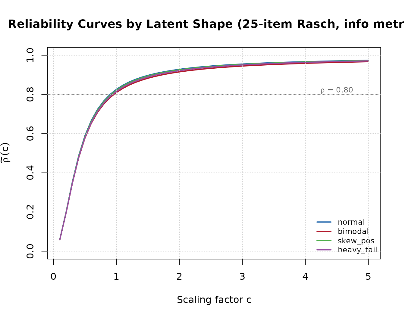

Reliability curves comparing how latent distribution shape changes the reliability-scale relationship.

The figure shows that all shapes can reach high reliability, but some require larger scaling factors c to compensate for the reduced average information when ability mass is spread away from the item difficulty region.

11.3 Calibrating Across Shapes

Use eqc_calibrate() with different latent_shape arguments to see how the calibrated c^* differs:

shapes_cal <- c("normal", "bimodal", "skew_pos", "heavy_tail", "uniform")
cal_results <- data.frame(
  shape = character(), c_star = numeric(),
  achieved_rho = numeric(), stringsAsFactors = FALSE
)

for (sh in shapes_cal) {
  res <- eqc_calibrate(
    target_rho = 0.80, n_items = 25, model = "rasch",
    latent_shape = sh, item_source = "parametric",
    reliability_metric = "info", M = 5000L, seed = 42
  )
  cal_results <- rbind(cal_results, data.frame(
    shape = sh, c_star = res$c_star,
    achieved_rho = res$achieved_rho, stringsAsFactors = FALSE
  ))
}

knitr::kable(
  cal_results,
  col.names = c("Shape", "c*", "Achieved rho"),
  digits = 4,
  caption = "Calibrated c* by latent shape (target rho = 0.80, 25-item Rasch)"
)

Calibrated c* by latent shape (target rho = 0.80, 25-item Rasch)
Shape	c*	Achieved rho
normal	0.8995	0.8
bimodal	0.9577	0.8
skew_pos	0.9132	0.8
heavy_tail	0.9365	0.8
uniform	0.9012	0.8

12. Using `sim_latentG()` with `eqc_calibrate()`

When using sim_latentG() as part of reliability-targeted simulation, specify the same parameters in eqc_calibrate():

# Calibrate for a bimodal population
eqc_result <- eqc_calibrate(
  target_rho = 0.80,
  n_items = 25,
  model = "rasch",
  latent_shape = "bimodal",
  latent_params = list(shape_params = list(delta = 0.8)),
  item_source = "parametric",
  reliability_metric = "info",
  M = 5000L,
  seed = 42
)

# Generate response data with the same distribution
sim_data <- simulate_response_data(
  result = eqc_result,
  n_persons = 1000,
  latent_shape = "bimodal",
  latent_params = list(shape_params = list(delta = 0.8)),
  seed = 123
)

cat(sprintf("Calibrated c* = %.4f, achieved rho = %.4f\n",
            eqc_result$c_star, eqc_result$achieved_rho))
#> Calibrated c* = 0.9577, achieved rho = 0.8000
cat(sprintf("Response data: %d persons x %d items\n",
            nrow(sim_data$response_matrix), ncol(sim_data$response_matrix)))
#> Response data: 1000 persons x 25 items

For the complete 6-step applied workflow, see vignette("applied-guide").

13. Summary of Shape Parameters

Shape	Parameter	Default	Range	Description
`bimodal`	`delta`	0.8	(0, 1)	Mode separation
`trimodal`	`w0`	1/3	(0, 1)	Weight of central component
	`m`	1.2	> 0	Location of side modes
`multimodal`	`m1`	0.5	> 0	Inner mode locations
	`m2`	1.3	> 0	Outer mode locations
	`w_inner`	0.30	(0, 0.5)	Weight of inner components
`skew_pos/neg`	`k`	4	> 0	Gamma shape (smaller = more skewed)
`heavy_tail`	`df`	5	> 2	Degrees of freedom (smaller = heavier)
`floor`	`w_floor`	0.3	(0, 1)	Weight at floor
	`m_floor`	-1.5	< 0	Floor location
`ceiling`	`w_ceil`	0.3	(0, 1)	Weight at ceiling
	`m_ceil`	1.5	> 0	Ceiling location

14. Practical Recommendations

14.1 Choosing a Shape

Research Question	Recommended Shape
Standard simulation	`normal`
Heterogeneous population	`bimodal`
Mixed ability levels	`trimodal` or `multimodal`
Selective samples	`skew_pos` or `skew_neg`
Robust estimation	`heavy_tail`
Easy/difficult tests	`ceiling` / `floor`
Sensitivity analysis	Compare multiple shapes

14.2 Sample Size Considerations

Choose quadrature size and replication sample size through a sensitivity or Monte Carlo precision analysis. Heavier tails and sparse mixture components often require larger draws, but no universal M or n threshold guarantees a desired error. Report the values used and, for calibration claims, evaluate the selected scale on independent theta draws.

14.3 Reproducibility

Always set a seed for reproducible results:

sim1 <- sim_latentG(n = 100, shape = "normal", seed = 42)
sim2 <- sim_latentG(n = 100, shape = "normal", seed = 42)
identical(sim1$theta, sim2$theta)  # TRUE
#> [1] TRUE

15. References

Lee, J.-H. (2026). Reliability-Targeted Simulation of Item Response Data: Solving the Inverse Design Problem. arXiv:2512.16012v2. https://doi.org/10.48550/arXiv.2512.16012

Baker, F. B., & Kim, S.-H. (2004). Item Response Theory: Parameter Estimation Techniques (2nd ed.). Marcel Dekker.

Paganin, S., et al. (2023). Computational strategies and estimation performance with Bayesian semiparametric item response theory models. Journal of Educational and Behavioral Statistics, 48(2), 147–188.

JoonHo Lee (jlee296@ua.edu)

2026-08-22

1. Overview

2. The Pre-Standardization Principle

2.1 Why This Matters

3. Basic Usage

4. Available Distribution Shapes

4.1 Standard Normal

4.2 Bimodal Distribution

4.3 Trimodal Distribution

4.4 Multimodal (Four Components)

4.5 Skewed Distributions

4.6 Heavy-Tailed Distribution

4.7 Light-Tailed (Platykurtic) Distribution

4.8 Uniform Distribution

4.9 Floor and Ceiling Effects

5. Comparing Multiple Shapes

6. Custom Mixture Distributions

7. Adjusting Location and Scale

8. Adding Covariate Effects

9. Working with the Output Object

9.1 Extracting Theta for Other Uses

10. Connection to IRT Framework

10.1 Marginal Reliability

10.2 Expected Test Information

10.3 Identifiability

11. How Latent Shape Affects Achievable Reliability

11.1 Feasibility Across Shapes

11.2 Reliability Curves Across Shapes

11.3 Calibrating Across Shapes

12. Using `sim_latentG()` with `eqc_calibrate()`

13. Summary of Shape Parameters

14. Practical Recommendations

14.1 Choosing a Shape

14.2 Sample Size Considerations

14.3 Reproducibility

15. References

Working with Latent Distributions

JoonHo Lee (jlee296@ua.edu)

2026-08-22

1. Overview

2. The Pre-Standardization Principle

2.1 Why This Matters

3. Basic Usage

4. Available Distribution Shapes

4.1 Standard Normal

4.2 Bimodal Distribution

4.3 Trimodal Distribution

4.4 Multimodal (Four Components)

4.5 Skewed Distributions

4.6 Heavy-Tailed Distribution

4.7 Light-Tailed (Platykurtic) Distribution

4.8 Uniform Distribution

4.9 Floor and Ceiling Effects

5. Comparing Multiple Shapes

6. Custom Mixture Distributions

7. Adjusting Location and Scale

8. Adding Covariate Effects

9. Working with the Output Object

9.1 Extracting Theta for Other Uses

10. Connection to IRT Framework

10.1 Marginal Reliability

10.2 Expected Test Information

10.3 Identifiability

11. How Latent Shape Affects Achievable Reliability

11.1 Feasibility Across Shapes

11.2 Reliability Curves Across Shapes

11.3 Calibrating Across Shapes

12. Using sim_latentG() with eqc_calibrate()

13. Summary of Shape Parameters

14. Practical Recommendations

14.1 Choosing a Shape

14.2 Sample Size Considerations

14.3 Reproducibility

15. References

12. Using `sim_latentG()` with `eqc_calibrate()`