Generating Realistic Item Parameters

1. Overview

Reading time: approximately 20–25 minutes.

The sim_item_params() function generates item parameters—difficulty \beta, discrimination \lambda, and, for the 3PL, lower asymptote g—for IRT simulation studies. It is designed with five key principles:

Realistic difficulties: Parametric defaults for portable simulations, with optional Item Response Warehouse (IRW) integration for empirically grounded difficulty distributions when the IRW package is installed.
Correlated parameters: Support for the empirically observed negative correlation between difficulty and discrimination.
Marginal control: The copula method keeps the sampled difficulty values unchanged while approximately targeting the requested discrimination marginal and dependence in a finite form.
Reliability targeting: A scale factor enables subsequent calibration for target reliability.
Explicit 3PL guessing: Lower asymptotes are generated independently of the global discrimination scale and retained in downstream results.

This vignette covers:

The difficulty-discrimination correlation
Basic usage (Rasch, 2PL, and 3PL)
Sources for difficulty generation
Methods for discrimination generation
Customizing discrimination parameters
Generating multiple test forms
Guessing distributions and the global scale parameter
Visualization
Extracting calibrated item parameters with coef()
Integration with calibration functions

For the complete calibration workflow, see vignette("applied-guide"). For theoretical details on how item parameters interact with reliability, see vignette("algorithm-eqc").

2. The Difficulty-Discrimination Correlation

A critical finding from psychometric research is that item difficulty and discrimination are negatively correlated in real assessments (Sweeney et al., 2022):

Easy items (\beta low) tend to have higher discrimination (\lambda high).
Difficult items (\beta high) tend to have lower discrimination (\lambda low).

This correlation, typically around \rho \approx -0.3, has important implications:

Ignoring it produces unrealistic simulation data.
Standard independent generation misses this structural feature.
The correlation affects test information functions.

sim_item_params() handles this by default using the copula method with \rho = -0.3.

3. Basic Usage

3.1 Rasch model

For the Rasch model, all discriminations are set to 1:

# Generate 25 Rasch items with parametric difficulties
items_rasch <- sim_item_params(
  n_items = 25,
  model   = "rasch",
  source  = "parametric",
  seed    = 42
)

print(items_rasch)
#> Item Parameters Object
#> ======================
#>   Model          : RASCH
#>   Source         : parametric
#>   Items per form : 25
#>   Number of forms: 1
#>   Scale factor   : 1.0000
#>   Centered       : Yes
#> 
#> Difficulty (beta):
#>   Mean: 0.0000, SD: 1.3064, Range: [-2.8440, 2.0991]

3.2 Two-parameter logistic (2PL) model

For the 2PL model, both difficulties and discriminations are generated:

# Generate 30 2PL items with correlated parameters
items_2pl <- sim_item_params(
  n_items = 30,
  model   = "2pl",
  source  = "parametric",
  method  = "copula",
  seed    = 42
)

print(items_2pl)
#> Item Parameters Object
#> ======================
#>   Model          : 2PL
#>   Source         : parametric
#>   Method         : copula
#>   Items per form : 30
#>   Number of forms: 1
#>   Scale factor   : 1.0000
#>   Centered       : Yes
#> 
#> Difficulty (beta):
#>   Mean: 0.0000, SD: 1.2550, Range: [-2.7250, 2.2181]
#> 
#> Discrimination (lambda, scaled):
#>   Mean: 1.0867, SD: 0.2885, Range: [0.4396, 1.7309]
#> 
#> Correlation (beta, log-lambda):
#>   Target (rho): -0.3000
#>   Achieved Pearson : -0.3611
#>   Achieved Spearman: -0.3784

The printed achieved correlation is one finite-form realization to compare with the default latent-Gaussian dependence input of -0.3; it is not constrained to equal that input.

3.3 Three-parameter logistic (3PL) model

The 3PL adds an item lower asymptote g_i while retaining the 2PL difficulty and discrimination generators. Supply its generator through guessing_params; the default is a fixed value of 0.20.

items_3pl <- sim_item_params(
  n_items = 30,
  model = "3pl",
  source = "parametric",
  method = "copula",
  guessing_params = list(distribution = "fixed", value = 0.20),
  seed = 42
)

items_3pl$data[1:6, c("beta", "lambda", "guessing")]
#>         beta    lambda guessing
#> 1  1.3023716 1.0310582      0.2
#> 2 -0.6332850 0.8507041      0.2
#> 3  0.2945416 1.4834002      0.2
#> 4  0.5642758 0.8467027      0.2
#> 5  0.3356815 1.1746005      0.2
#> 6 -0.1747114 1.1006382      0.2

Available guessing generators are:

`distribution`	Fields	Meaning
`"fixed"`	`value`	One scalar (recycled) or one value per item
`"beta"`	`shape1`, `shape2`	Beta-distributed values on [0,1)
`"uniform"`	`min`, `max`	Uniform values with 0 \leq \min < \max < 1

For source = "custom", put the lower asymptotes in custom_params$guessing instead of guessing_params. Every g_i must be finite and satisfy 0 \leq g_i < 1.

# With g = 0, the 3PL is exactly nested in the 2PL. The same seed also
# produces the same beta and lambda draws because fixed guessing uses no RNG.
items_2pl_g0 <- sim_item_params(12, model = "2pl", seed = 91)
items_3pl_g0 <- sim_item_params(
  12, model = "3pl",
  guessing_params = list(distribution = "fixed", value = 0),
  seed = 91
)
stopifnot(
  identical(items_2pl_g0$data$beta, items_3pl_g0$data$beta),
  identical(items_2pl_g0$data$lambda, items_3pl_g0$data$lambda),
  all(items_3pl_g0$data$guessing == 0)
)

4. Sources for Difficulty Generation

sim_item_params() supports four sources for generating item difficulties.

4.1 Optional IRW (Item Response Warehouse)

IRW is an optional external source for empirically grounded simulations. It can provide difficulty distributions based on real assessment items when the IRW package is installed. The default, dependency-free source remains source = "parametric".

if (requireNamespace("irw", quietly = TRUE)) {
  items_irw <- sim_item_params(
    n_items = 25,
    model   = "rasch",
    source  = "irw",
    seed    = 42
  )

  summary(items_irw$data$beta)
}

4.2 Parametric

Generate difficulties from a parametric distribution:

# Normal distribution (default)
items_normal <- sim_item_params(
  n_items = 25,
  model   = "rasch",
  source  = "parametric",
  difficulty_params = list(mu = 0, sigma = 1, distribution = "normal"),
  seed    = 42
)

# Uniform distribution
items_uniform <- sim_item_params(
  n_items = 25,
  model   = "rasch",
  source  = "parametric",
  difficulty_params = list(mu = 0, sigma = 1, distribution = "uniform"),
  seed    = 42
)

par(mfrow = c(1, 2))
hist(items_normal$data$beta, breaks = 12, col = pal$primary,
     border = "white", main = "Normal Difficulties", xlab = expression(beta))
hist(items_uniform$data$beta, breaks = 12, col = pal$secondary,
     border = "white", main = "Uniform Difficulties", xlab = expression(beta))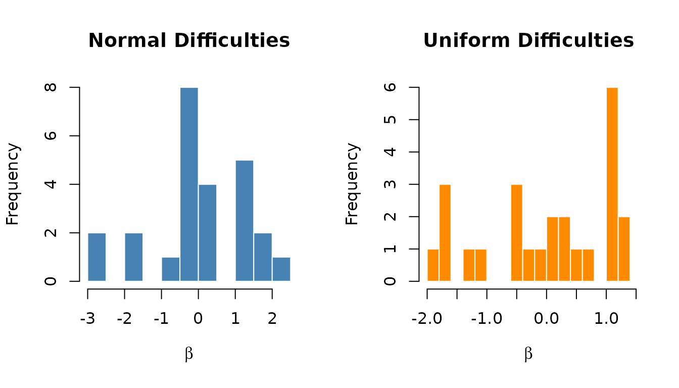

Side-by-side plots comparing parametric item difficulty and discrimination distributions.

par(mfrow = c(1, 1))

4.3 Hierarchical

Joint bivariate normal generation following Glas & van der Linden (2003). Both \log(\lambda) and \beta are drawn from a multivariate normal:

\begin{pmatrix} \log(\lambda_i) \\ \beta_i \end{pmatrix} \sim N\!\left( \begin{pmatrix} \mu_\lambda \\ \mu_\beta \end{pmatrix}, \begin{pmatrix} \tau_\lambda^2 & \rho \tau_\lambda \tau_\beta \\ \rho \tau_\lambda \tau_\beta & \tau_\beta^2 \end{pmatrix} \right)

items_hier <- sim_item_params(
  n_items = 25,
  model   = "2pl",
  source  = "hierarchical",
  hierarchical_params = list(
    mu  = c(0, 0),
    tau = c(0.25, 1),
    rho = -0.3
  ),
  seed = 42
)

print(items_hier)
#> Item Parameters Object
#> ======================
#>   Model          : 2PL
#>   Source         : hierarchical
#>   Items per form : 25
#>   Number of forms: 1
#>   Scale factor   : 1.0000
#>   Centered       : Yes
#> 
#> Difficulty (beta):
#>   Mean: -0.0000, SD: 1.3077, Range: [-2.8627, 2.1086]
#> 
#> Discrimination (lambda, scaled):
#>   Mean: 1.0776, SD: 0.2710, Range: [0.7199, 1.8119]
#> 
#> Correlation (beta, log-lambda):
#>   Target (rho): -0.3000
#>   Achieved Pearson : -0.3451
#>   Achieved Spearman: -0.3746

4.4 Custom

Supply your own parameters directly:

# Custom difficulties and discriminations
items_custom <- sim_item_params(
  n_items = 10,
  model   = "2pl",
  source  = "custom",
  custom_params = list(
    beta   = seq(-2, 2, length.out = 10),
    lambda = rep(1.2, 10)
  ),
  seed = 42
)

items_custom$data
#>    form_id item_id       beta lambda lambda_unscaled
#> 1        1       1 -2.0000000    1.2             1.2
#> 2        1       2 -1.5555556    1.2             1.2
#> 3        1       3 -1.1111111    1.2             1.2
#> 4        1       4 -0.6666667    1.2             1.2
#> 5        1       5 -0.2222222    1.2             1.2
#> 6        1       6  0.2222222    1.2             1.2
#> 7        1       7  0.6666667    1.2             1.2
#> 8        1       8  1.1111111    1.2             1.2
#> 9        1       9  1.5555556    1.2             1.2
#> 10       1      10  2.0000000    1.2             1.2

A custom 3PL form requires all three item vectors. A scalar guessing value is accepted and recycled, but an explicit vector is often clearer when freezing a form for calibration:

items_custom_3pl <- sim_item_params(
  n_items = 10,
  model = "3pl",
  source = "custom",
  custom_params = list(
    beta = seq(-2, 2, length.out = 10),
    lambda = rep(1.2, 10),
    guessing = rep(0.20, 10)
  ),
  seed = 42
)
items_custom_3pl$data
#>    form_id item_id       beta lambda lambda_unscaled guessing
#> 1        1       1 -2.0000000    1.2             1.2      0.2
#> 2        1       2 -1.5555556    1.2             1.2      0.2
#> 3        1       3 -1.1111111    1.2             1.2      0.2
#> 4        1       4 -0.6666667    1.2             1.2      0.2
#> 5        1       5 -0.2222222    1.2             1.2      0.2
#> 6        1       6  0.2222222    1.2             1.2      0.2
#> 7        1       7  0.6666667    1.2             1.2      0.2
#> 8        1       8  1.1111111    1.2             1.2      0.2
#> 9        1       9  1.5555556    1.2             1.2      0.2
#> 10       1      10  2.0000000    1.2             1.2      0.2

You can also provide functions that generate parameters:

items_custom_fn <- sim_item_params(
  n_items = 20,
  model   = "2pl",
  source  = "custom",
  custom_params = list(
    beta   = function(n) rnorm(n, 0, 1.5),
    lambda = function(n) rlnorm(n, 0, 0.3)
  ),
  seed = 42
)

5. Methods for Discrimination Generation

When using source = "irw" or source = "parametric" with model = "2pl" or model = "3pl", you can choose how discriminations are generated. The default is method = "copula", and three methods are available.

5.1 Copula method (recommended)

The rank-based Gaussian copula method leaves the sampled difficulty values unchanged while approximately targeting the requested discrimination marginal and dependence in a finite form. The supplied rho is a latent Gaussian dependence parameter; realized Pearson and Spearman correlations are stochastic and are not guaranteed to equal it.

Algorithm:

Transform \beta to uniform scores: u = \{\text{rank}(\beta)-0.5\}/n.
Transform to normal: z_\beta = \Phi^{-1}(u).
Generate correlated normal: z_\lambda = \rho \cdot z_\beta + \sqrt{1-\rho^2} \cdot z_{\text{indep}}.
Transform to uniform: v = \Phi(z_\lambda).
Transform to log-normal: \lambda = \exp(\mu + \sigma \cdot \Phi^{-1}(v)).

items_copula <- sim_item_params(
  n_items = 100,
  model   = "2pl",
  source  = "parametric",
  method  = "copula",
  discrimination_params = list(
    mu_log    = 0,
    sigma_log = 0.3,
    rho       = -0.3
  ),
  seed = 42
)

# Check achieved correlation
cat(sprintf("Target rho: -0.30\n"))
#> Target rho: -0.30
cat(sprintf("Achieved Spearman: %.3f\n",
            items_copula$achieved$overall$cor_spearman_pooled))
#> Achieved Spearman: -0.237

Why copula is recommended:

Preserves the exact difficulty distribution.
Approximately targets a log-normal discrimination marginal in a finite form.
Uses rho as a latent-Gaussian dependence input; realized Pearson and Spearman correlations are stochastic and should be inspected.
Works well with any difficulty distribution shape.

5.2 Conditional method

Uses conditional normal regression:

\log(\lambda_i) \mid \beta_i \sim N\!\left(\mu_{\log} + \rho \cdot \sigma_{\log} \cdot z_{\beta_i}, \; \sigma_{\log}\sqrt{1-\rho^2}\right)

items_cond <- sim_item_params(
  n_items = 100,
  model   = "2pl",
  source  = "parametric",
  method  = "conditional",
  discrimination_params = list(rho = -0.3),
  seed    = 42
)

cat(sprintf("Achieved Pearson:  %.3f\n",
            items_cond$achieved$overall$cor_pearson_pooled))
#> Achieved Pearson:  -0.302
cat(sprintf("Achieved Spearman: %.3f\n",
            items_cond$achieved$overall$cor_spearman_pooled))
#> Achieved Spearman: -0.310

Note: The conditional method assumes linear relationships and normal errors. When empirical or other non-normal difficulties are used, achieved correlations may differ from targets.

5.3 Independent method

Generates discriminations independently of difficulties (no correlation):

items_indep <- sim_item_params(
  n_items = 100,
  model   = "2pl",
  source  = "parametric",
  method  = "independent",
  seed    = 42
)

cat(sprintf("Achieved correlation: %.3f (expected: ~0)\n",
            items_indep$achieved$overall$cor_spearman_pooled))
#> Achieved correlation: 0.051 (expected: ~0)

6. Customizing Discrimination Parameters

The discrimination_params list controls the log-normal distribution of discriminations:

# Higher average discrimination
items_high_disc <- sim_item_params(
  n_items = 30,
  model   = "2pl",
  source  = "parametric",
  method  = "copula",
  discrimination_params = list(
    mu_log    = 0.3,
    sigma_log = 0.25,
    rho       = -0.3
  ),
  seed = 42
)

cat(sprintf("Mean lambda: %.3f\n", mean(items_high_disc$data$lambda)))
#> Mean lambda: 1.440
cat(sprintf("SD lambda:   %.3f\n", sd(items_high_disc$data$lambda)))
#> SD lambda:   0.321

6.1 Understanding the parameters

Parameter	Default	Description
`mu_log`	0	Mean of \log(\lambda). \mathbb{E}[\lambda] \approx \exp(\mu_{\log} + \sigma_{\log}^2/2)
`sigma_log`	0.3	SD of \log(\lambda). Controls heterogeneity across items
`rho`	-0.3	Latent-Gaussian dependence input for \beta and \log(\lambda); finite-form correlations are stochastic

7. Generating Multiple Test Forms

Generate multiple parallel forms with independent item samples:

items_5forms <- sim_item_params(
  n_items = 20,
  model   = "2pl",
  source  = "parametric",
  method  = "copula",
  n_forms = 5,
  seed    = 42
)

cat(sprintf("Total items: %d\n", nrow(items_5forms$data)))
#> Total items: 100
cat(sprintf("Items per form: %d\n", items_5forms$n_items))
#> Items per form: 20
cat(sprintf("Number of forms: %d\n", items_5forms$n_forms))
#> Number of forms: 5

# View first few rows
head(items_5forms$data, 10)
#>    form_id item_id       beta    lambda lambda_unscaled
#> 1        1       1  1.1790384 1.0473137       1.0473137
#> 2        1       2 -0.7566182 1.3308590       1.3308590
#> 3        1       3  0.1712084 1.3372084       1.3372084
#> 4        1       4  0.4409426 0.8163263       0.8163263
#> 5        1       5  0.2123483 1.1359716       1.1359716
#> 6        1       6 -0.2980445 0.6295821       0.6295821
#> 7        1       7  1.3196020 0.7203419       0.7203419
#> 8        1       8 -0.2865791 0.7973245       0.7973245
#> 9        1       9  1.8265037 0.4402291       0.4402291
#> 10       1      10 -0.2546341 1.0161096       1.0161096

7.1 Per-form statistics

for (f in 1:3) {
  stats <- items_5forms$achieved$by_form[[f]]
  cat(sprintf("Form %d: beta_mean=%.3f, lambda_mean=%.3f, cor=%.3f\n",
              f, stats$beta_mean, stats$lambda_mean, stats$cor_spearman))
}
#> Form 1: beta_mean=-0.000, lambda_mean=0.992, cor=-0.382
#> Form 2: beta_mean=-0.000, lambda_mean=1.063, cor=-0.356
#> Form 3: beta_mean=0.000, lambda_mean=1.031, cor=-0.463

8. The Scale Parameter

The scale parameter is central to the reliability-targeted framework. It multiplies all discriminations by a constant factor:

\lambda_i^* = c \cdot \lambda_{i,0}

where \lambda_{i,0} is the baseline discrimination and c is the scale factor.

For a 3PL item, the full response probability is

P(Y_i=1\mid\theta)=g_i+(1-g_i) \operatorname{logit}^{-1}\{c\lambda_{i,0}(\theta-\beta_i)\}.

Thus, scale = c multiplies only discrimination. It does not scale the lower asymptote: use guessing_params (or custom_params$guessing) to define g_i. Calibration functions estimate this same global c while holding the generated \beta_i and g_i fixed.

# Baseline (scale = 1)
items_base <- sim_item_params(
  n_items = 25, model = "2pl", source = "parametric",
  scale = 1, seed = 42
)

# Scaled up (scale = 1.5)
items_scaled <- sim_item_params(
  n_items = 25, model = "2pl", source = "parametric",
  scale = 1.5, seed = 42
)

cat(sprintf("Baseline mean lambda: %.3f\n", mean(items_base$data$lambda)))
#> Baseline mean lambda: 0.994
cat(sprintf("Scaled mean lambda:   %.3f\n", mean(items_scaled$data$lambda)))
#> Scaled mean lambda:   1.491
cat(sprintf("Ratio: %.2f\n",
            mean(items_scaled$data$lambda) / mean(items_base$data$lambda)))
#> Ratio: 1.50

8.1 Unscaled lambda

The output always includes lambda_unscaled for reference:

head(items_scaled$data[, c("lambda", "lambda_unscaled")])
#>      lambda lambda_unscaled
#> 1 1.6312287       1.0874858
#> 2 1.4873989       0.9915993
#> 3 0.6383717       0.4255811
#> 4 1.0951612       0.7301075
#> 5 1.6391847       1.0927898
#> 6 1.5991754       1.0661169

# Verify relationship
all.equal(
  items_scaled$data$lambda,
  items_scaled$data$lambda_unscaled * items_scaled$scale
)
#> [1] TRUE

The distinction is directly checkable for a 3PL form:

items_3pl_scaled <- sim_item_params(
  n_items = 12,
  model = "3pl",
  scale = 1.5,
  guessing_params = list(distribution = "fixed", value = 0.20),
  seed = 42
)
stopifnot(
  all.equal(
    items_3pl_scaled$data$lambda,
    1.5 * items_3pl_scaled$data$lambda_unscaled
  ),
  all(items_3pl_scaled$data$guessing == 0.20)
)

9. Centering Difficulties

By default, difficulties are centered to sum to zero (for model identification):

# Default: centered
items_centered <- sim_item_params(
  n_items = 25, model = "rasch", source = "parametric",
  center_difficulties = TRUE, seed = 42
)

# Uncentered
items_uncentered <- sim_item_params(
  n_items = 25, model = "rasch", source = "parametric",
  center_difficulties = FALSE, seed = 42
)

cat(sprintf("Centered mean:   %.6f\n", mean(items_centered$data$beta)))
#> Centered mean:   0.000000
cat(sprintf("Uncentered mean: %.6f\n", mean(items_uncentered$data$beta)))
#> Uncentered mean: 0.187536

10. Visualization

The plot() method provides diagnostic visualizations:

items_viz <- sim_item_params(
  n_items = 50, model = "2pl", source = "parametric",
  method = "copula", seed = 42
)

# Scatter plot with regression line
plot(items_viz, type = "scatter")
#> `geom_smooth()` using formula = 'y ~ x'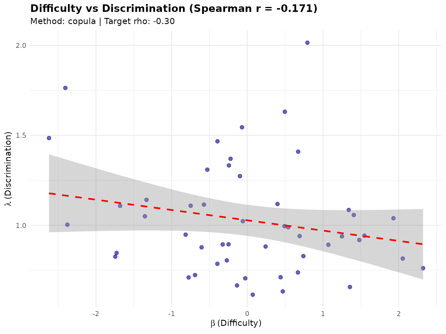

Scatter plot of item difficulty and discrimination with diagnostic reference patterns.

# Density plots
plot(items_viz, type = "density")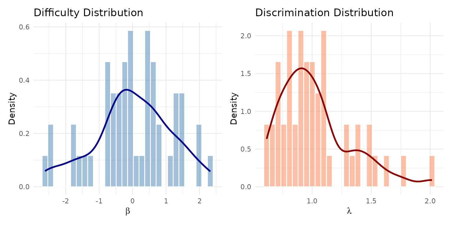

Density plots of simulated item difficulty and discrimination parameters.

11. Extracting Calibrated Item Parameters with `coef()`

After running eqc_calibrate() or sac_calibrate(), the coef() method extracts a tidy data frame of all item parameters—including both baseline and calibrated (scaled) discriminations.

11.1 From an EQC result

eqc_result <- eqc_calibrate(
  target_rho  = 0.85,
  n_items     = 25,
  model       = "rasch",
  item_source = "parametric",
  reliability_metric = "info",
  M           = 5000L,
  seed        = 42
)

# Extract calibrated item parameters
item_table <- coef(eqc_result)
head(item_table)
#>   item_id         beta lambda_base lambda_scaled   c_star
#> 1       1  0.197732269           1      1.119883 1.119883
#> 2       2  1.096799859           1      1.119883 1.119883
#> 3       3  0.436545084           1      1.119883 1.119883
#> 4       4 -0.013038730           1      1.119883 1.119883
#> 5       5 -0.199801302           1      1.119883 1.119883
#> 6       6  0.007700326           1      1.119883 1.119883

Each row contains:

Column	Description
`item_id`	Item identifier (1 to I)
`beta`	Item difficulty
`lambda_base`	Baseline (unscaled) discrimination
`lambda_scaled`	Calibrated discrimination: \lambda_{\text{base}} \times c^*
`c_star`	The calibrated scaling factor (constant across items)
`guessing`	3PL lower asymptote; present for 3PL results and not scaled by c^*

11.2 Summary statistics from coef output

cat(sprintf("Number of items:       %d\n", nrow(item_table)))
#> Number of items:       25
cat(sprintf("Difficulty range:      [%.3f, %.3f]\n",
            min(item_table$beta), max(item_table$beta)))
#> Difficulty range:      [-2.170, 1.450]
cat(sprintf("Difficulty mean:       %.4f\n", mean(item_table$beta)))
#> Difficulty mean:       0.0000
cat(sprintf("Difficulty SD:         %.4f\n", sd(item_table$beta)))
#> Difficulty SD:         0.8606
cat(sprintf("Calibrated c*:         %.4f\n", item_table$c_star[1]))
#> Calibrated c*:         1.1199
cat(sprintf("Scaled discrimination: %.4f (all equal for Rasch)\n",
            item_table$lambda_scaled[1]))
#> Scaled discrimination: 1.1199 (all equal for Rasch)

11.3 From a SAC result

The same coef() interface works for SAC results:

sac_result <- sac_calibrate(
  target_rho        = 0.85,
  n_items           = 25,
  model             = "rasch",
  reliability_metric = "info",
  c_init            = eqc_result,
  resample_items    = FALSE,
  n_iter            = 200L,
  M_per_iter        = 500L,
  M_pre             = 5000L,
  seed              = 42
)

sac_items <- coef(sac_result)
head(sac_items)
#>   item_id         beta lambda_base lambda_scaled   c_star
#> 1       1  0.197732269           1      1.119847 1.119847
#> 2       2  1.096799859           1      1.119847 1.119847
#> 3       3  0.436545084           1      1.119847 1.119847
#> 4       4 -0.013038730           1      1.119847 1.119847
#> 5       5 -0.199801302           1      1.119847 1.119847
#> 6       6  0.007700326           1      1.119847 1.119847

11.4 Comparing EQC and SAC item parameters

cat(sprintf("EQC c*: %.4f\n", item_table$c_star[1]))
#> EQC c*: 1.1199
cat(sprintf("SAC c*: %.4f\n", sac_items$c_star[1]))
#> SAC c*: 1.1198
cat(sprintf("Difference: %.4f (%.2f%%)\n",
            abs(item_table$c_star[1] - sac_items$c_star[1]),
            100 * abs(item_table$c_star[1] - sac_items$c_star[1]) / item_table$c_star[1]))
#> Difference: 0.0000 (0.00%)

11.5 Exporting to CSV

# Save calibrated item parameters for use in other software
output_file <- file.path(tempdir(), "calibrated_items.csv")
write.csv(coef(eqc_result), file = output_file, row.names = FALSE)
output_file

11.6 Using coef output with 2PL models

With 2PL models, the baseline discriminations vary across items, and coef() makes it easy to see both the original and scaled values:

eqc_2pl <- eqc_calibrate(
  target_rho  = 0.80,
  n_items     = 20,
  model       = "2pl",
  item_source = "parametric",
  reliability_metric = "info",
  M           = 5000L,
  seed        = 42
)

items_2pl_df <- coef(eqc_2pl)
head(items_2pl_df, 10)
#>    item_id         beta lambda_base lambda_scaled   c_star
#> 1        1  0.217684472   1.1349399     1.0243650 0.902572
#> 2        2  1.116752062   0.8790623     0.7934170 0.902572
#> 3        3  0.456497288   0.6153466     0.5553947 0.902572
#> 4        4  0.006913473   0.9368403     0.8455659 0.902572
#> 5        5 -0.179849098   1.6009565     1.4449786 0.902572
#> 6        6  0.027652529   0.6234454     0.5627044 0.902572
#> 7        7  1.040020929   0.9415274     0.8497963 0.902572
#> 8        8  0.357576547   1.4926448     1.3472194 0.902572
#> 9        9 -0.342317758   0.9401472     0.8485505 0.902572
#> 10      10 -0.073909889   1.1890902     1.0732396 0.902572

plot(items_2pl_df$beta, items_2pl_df$lambda_scaled,
     pch = 16, col = pal$primary, cex = 1.2,
     xlab = expression(beta), ylab = expression(lambda^"*"),
     main = "Calibrated Item Parameters (2PL)")
abline(lm(lambda_scaled ~ beta, data = items_2pl_df),
       col = pal$accent, lty = 2, lwd = 1.5)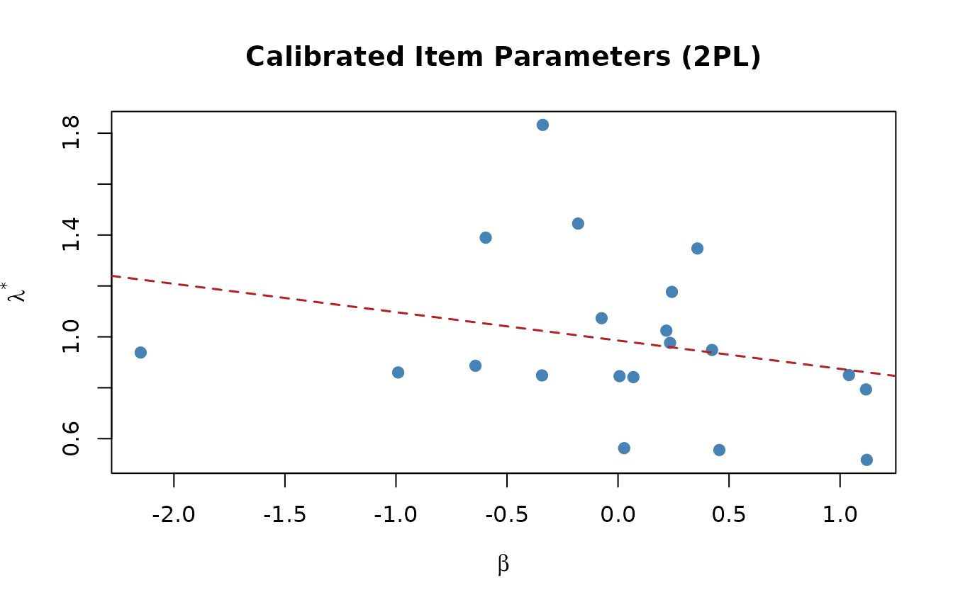

Scatter plot of calibrated 2PL item difficulties and scaled discriminations.

11.7 Using `coef()` with a 3PL model

For 3PL results, the coefficient table retains the fixed lower asymptotes:

eqc_3pl <- eqc_calibrate(
  target_rho = 0.70,
  n_items = 12,
  model = "3pl",
  item_params = list(
    guessing_params = list(distribution = "fixed", value = 0.20)
  ),
  reliability_metric = "info",
  M = 2000L,
  seed = 310
)

items_3pl_df <- coef(eqc_3pl)
items_3pl_df[1:6, c(
  "beta", "lambda_base", "lambda_scaled", "guessing", "c_star"
)]
#>         beta lambda_base lambda_scaled guessing   c_star
#> 1  1.8982922   0.5502690     0.7324069      0.2 1.330998
#> 2 -1.1698188   1.1766709     1.5661465      0.2 1.330998
#> 3 -0.4374418   1.3966358     1.8589194      0.2 1.330998
#> 4  0.6494564   1.7728133     2.3596108      0.2 1.330998
#> 5 -0.4444675   1.1381177     1.5148323      0.2 1.330998
#> 6  2.2486312   0.9185855     1.2226353      0.2 1.330998
stopifnot(all(items_3pl_df$guessing == 0.20))

12. Integration with eqc_calibrate

In the reliability-targeted simulation framework, sim_item_params() is called internally by eqc_calibrate(). You specify item generation settings through the item_source and item_params arguments:

# EQC automatically calls sim_item_params internally
eqc_result_full <- eqc_calibrate(
  target_rho  = 0.80,
  n_items     = 25,
  model       = "2pl",
  item_source = "parametric",
  reliability_metric = "info",
  item_params = list(
    discrimination_params = list(
      mu_log    = 0,
      sigma_log = 0.3,
      rho       = -0.3
    )
  ),
  M    = 5000L,
  seed = 42
)

cat(sprintf("c* = %.4f, achieved rho = %.4f\n",
            eqc_result_full$c_star, eqc_result_full$achieved_rho))
#> c* = 0.8637, achieved rho = 0.8000

For a 3PL calibration, the guessing generator is nested inside item_params because eqc_calibrate() passes that list to sim_item_params():

eqc_3pl_generated <- eqc_calibrate(
  target_rho = 0.70,
  n_items = 12,
  model = "3pl",
  item_source = "parametric",
  item_params = list(
    discrimination_params = list(rho = -0.3),
    guessing_params = list(distribution = "beta", shape1 = 5, shape2 = 17)
  ),
  reliability_metric = "info",
  M = 2000L,
  seed = 311
)
summary(coef(eqc_3pl_generated)$guessing)
#>    Min. 1st Qu.  Median    Mean 3rd Qu.    Max. 
#>  0.1344  0.2180  0.2312  0.2421  0.2910  0.3192

EQC calibrates the one form stored in its result (item_scope = "fixed_form"). SAC can either reuse that form with resample_items = FALSE or target a generator-level item superpopulation with resample_items = TRUE. Those are different estimands; only the fixed-form, same-metric run can use an EQC result as a comparable warm start.

12.1 Accessing calibrated items

After calibration, you can access both baseline and calibrated item parameters:

# Baseline items (scale = 1)
items_base_obj <- eqc_result_full$items_base

# Calibrated items (scale = c*)
items_calib_obj <- eqc_result_full$items_calib

# The calibration factor
c_star <- eqc_result_full$c_star

cat(sprintf("Baseline scale:    %d\n", items_base_obj$scale))
#> Baseline scale:    1
cat(sprintf("Calibrated scale:  %.4f\n", items_calib_obj$scale))
#> Calibrated scale:  0.8637

13. Comparison of Methods

Compare the three discrimination generation methods:

methods <- c("copula", "conditional", "independent")
results <- list()

for (m in methods) {
  results[[m]] <- sim_item_params(
    n_items = 200, model = "2pl", source = "parametric",
    method = m,
    discrimination_params = list(rho = -0.4),
    seed = 123
  )
}

# Compare achieved correlations
cat("Method Comparison (target rho = -0.4):\n")
#> Method Comparison (target rho = -0.4):
cat("======================================\n")
#> ======================================
for (m in methods) {
  cat(sprintf("%-12s: Pearson = %+.3f, Spearman = %+.3f\n",
              m,
              results[[m]]$achieved$overall$cor_pearson_pooled,
              results[[m]]$achieved$overall$cor_spearman_pooled))
}
#> copula      : Pearson = -0.465, Spearman = -0.452
#> conditional : Pearson = -0.422, Spearman = -0.416
#> independent : Pearson = -0.028, Spearman = -0.046

The copula method usually tracks the requested direction and magnitude of dependence more closely than the alternatives in this example, but the finite-form correlation remains stochastic and is not constrained to equal rho.

14. Working with the Output Object

The item_params object contains rich information:

items <- sim_item_params(
  n_items = 25, model = "2pl", source = "parametric", seed = 42
)

# Structure
names(items)
#>  [1] "data"     "model"    "source"   "method"   "n_items"  "n_forms" 
#>  [7] "scale"    "centered" "params"   "achieved"

# Extract as data frame
df <- as.data.frame(items)
head(df)
#>   form_id item_id       beta    lambda lambda_unscaled
#> 1       1       1  1.1834223 1.0874858       1.0874858
#> 2       1       2 -0.7522343 0.9915993       0.9915993
#> 3       1       3  0.1755922 0.4255811       0.4255811
#> 4       1       4  0.4453264 0.7301075       0.7301075
#> 5       1       5  0.2167322 1.0927898       1.0927898
#> 6       1       6 -0.2936607 1.0661169       1.0661169

# Achieved statistics
items$achieved$overall
#> $n_total
#> [1] 25
#> 
#> $beta_mean
#> [1] 0
#> 
#> $beta_sd
#> [1] 1.306365
#> 
#> $lambda_mean
#> [1] 0.99377
#> 
#> $lambda_sd
#> [1] 0.3251601
#> 
#> $cor_pearson_pooled
#> [1] -0.2580066
#> 
#> $cor_spearman_pooled
#> [1] -0.3038462

15. Summary Tables

15.1 Sources

Source	Description	Best For
`parametric`	Normal/uniform difficulties	Controlled experiments and dependency-free examples
`irw`	Optional Item Response Warehouse integration	Empirically grounded simulations when IRW is installed
`hierarchical`	Joint MVN generation	Bayesian framework
`custom`	User-supplied parameters	Specific scenarios

For 3PL models, every source above can be paired with guessing_params, except that source = "custom" uses custom_params$guessing.

15.2 Methods

Method	Difficulty Values	Dependence Input	Notes
`copula`	Preserved exactly	Latent Gaussian `rho`	Approximate discrimination marginal and stochastic realized correlations; recommended
`conditional`	Preserved exactly	Conditional-regression `rho`	Assumes standardized difficulty enters linearly
`independent`	Preserved exactly	None	Realized finite-form correlation fluctuates around zero

16. Practical Recommendations

16.1 For realistic simulations

if (requireNamespace("irw", quietly = TRUE)) {
  items <- sim_item_params(
    n_items = 30, model = "2pl",
    source = "irw",
    method = "copula",
    discrimination_params = list(mu_log = 0, sigma_log = 0.3, rho = -0.3),
    seed = 42
  )
}

16.2 For controlled experiments

items <- sim_item_params(
  n_items = 25, model = "2pl",
  source = "parametric",
  difficulty_params = list(mu = 0, sigma = 1),
  method = "conditional",
  discrimination_params = list(mu_log = 0, sigma_log = 0.25, rho = 0),
  seed = 42
)

16.3 For Bayesian frameworks

items <- sim_item_params(
  n_items = 25, model = "2pl",
  source = "hierarchical",
  hierarchical_params = list(mu = c(0, 0), tau = c(0.3, 1), rho = -0.3),
  seed = 42
)

16.4 For controlled 3PL experiments

items <- sim_item_params(
  n_items = 25,
  model = "3pl",
  source = "parametric",
  method = "copula",
  discrimination_params = list(mu_log = 0, sigma_log = 0.25, rho = -0.3),
  guessing_params = list(distribution = "fixed", value = 0.20),
  scale = 1,
  seed = 42
)

Use scale = 1 when defining the baseline form, then let EQC or SAC estimate the global discrimination multiplier. Keep guessing_params fixed across conditions unless lower-asymptote variation is itself part of the design.

References

Lee, J.-H. (2026). Reliability-Targeted Simulation of Item Response Data: Solving the Inverse Design Problem. arXiv:2512.16012v2. https://doi.org/10.48550/arXiv.2512.16012

Glas, C. A. W., & van der Linden, W. J. (2003). Computerized adaptive testing with item cloning. Applied Psychological Measurement, 27(4), 247–261.

Sweeney, S. M., et al. (2022). An investigation of the nature and consequence of the relationship between IRT difficulty and discrimination. Educational Measurement: Issues and Practice, 41(4), 50–67.

Zhang, L., Liu, Y., Molenaar, D., & Domingue, B. (2025). Realistic Simulation of Item Difficulties. PsyArXiv. https://osf.io/preprints/psyarxiv/jbhxy_v3/

JoonHo Lee (jlee296@ua.edu)

2026-08-22