Case Studies: Publication-Ready Simulation Templates

Overview

Reading time: approximately 30–35 minutes.

This vignette presents three self-contained case studies, each with a research question, factorial design, executable code, computed results, and a publication-ready methods paragraph. Every case study can serve as a starting template for your own simulation work.

Case Study	Research Question	Key Factors
1	Does the 2PL model recover difficulty better than Rasch when reliability is held constant?	Model (Rasch vs. 2PL) x Reliability
2	How does latent distribution misspecification affect parameter recovery at controlled reliability?	Generating distribution x Calibration distribution
3	What minimum sample size is needed for stable difficulty recovery?	Sample size (N) at fixed reliability

Each case study follows the same five-step structure:

Research question: a precise, falsifiable question.
Design: a factorial layout with all factors and levels.
Code: executable R code using IRTsimrel.
Results: tables and figures computed from eval=TRUE code.
Methods text: a publication-ready paragraph.

Prerequisites: familiarity with eqc_calibrate() and simulate_response_data(). See vignette("introduction") and vignette("simulation-design") for background.

These examples intentionally focus on Rasch/2PL comparisons; that limited factorial design is not a package limitation. The general template also accepts model = "3pl" when a scientifically justified lower-asymptote specification is supplied.

Case Study 1: Model Comparison Under Controlled Reliability

Research question

Does the 2PL model recover item difficulty parameters better than the Rasch model when marginal reliability is held constant?

Without reliability control, any observed difference in recovery accuracy could be an artifact of differing data quality. By fixing reliability, we isolate the effect of model structure on parameter recovery.

This is a fundamental question in IRT methodology. The 2PL model has more parameters to estimate, which may affect the precision of difficulty estimates even when the overall data quality (as measured by reliability) is equivalent.

Design

Factor	Levels
Model	Rasch, 2PL
Reliability	0.60, 0.70, 0.80
Test length	20 items (fixed)
N persons	300 (fixed)
Replications	5 (for demonstration; use 500+ in practice)

cs1_design <- expand.grid(
  model       = c("rasch", "2pl"),
  target_rho  = c(0.60, 0.70, 0.80),
  stringsAsFactors = FALSE
)
n_items  <- 20
n_persons <- 300
R <- 5  # Use R = 500+ for a real study

cat(sprintf("Design cells: %d\n", nrow(cs1_design)))
#> Design cells: 6
cat(sprintf("Total data sets: %d\n", nrow(cs1_design) * R))
#> Total data sets: 30

Step 1: Feasibility screening

Before calibration, verify that all target reliabilities are achievable:

for (mod in c("rasch", "2pl")) {
  feas <- check_feasibility(
    n_items      = n_items,
    model        = mod,
    item_source  = "parametric",
    target_rho   = max(cs1_design$target_rho),
    M            = 5000L,
    seed         = 42,
    verbose      = FALSE
  )
  cat(sprintf("  %s: achievable rho_tilde = [%.3f, %.3f]\n",
              toupper(mod), feas$rho_range_info[1], feas$rho_range_info[2]))
}
#>   RASCH: achievable rho_tilde = [0.048, 0.985]
#>   2PL: achievable rho_tilde = [0.062, 0.987]

All target reliabilities (0.60, 0.70, 0.80) are within range.

Step 2: Calibrate all conditions

cs1_calib <- vector("list", nrow(cs1_design))

for (i in seq_len(nrow(cs1_design))) {
  d <- cs1_design[i, ]
  cs1_calib[[i]] <- eqc_calibrate(
    target_rho   = d$target_rho,
    n_items      = n_items,
    model        = d$model,
    item_source  = "parametric",
    reliability_metric = "info",
    M            = 5000L,
    seed         = 42,
    verbose      = FALSE
  )
}

# Verify calibration accuracy
cs1_design$achieved_rho <- vapply(cs1_calib, function(r) r$achieved_rho, numeric(1))
cs1_design$c_star       <- vapply(cs1_calib, function(r) r$c_star, numeric(1))

print(cs1_design)
#>   model target_rho achieved_rho    c_star
#> 1 rasch        0.6    0.6000000 0.5754710
#> 2   2pl        0.6    0.6000001 0.5060875
#> 3 rasch        0.7    0.7000000 0.7380684
#> 4   2pl        0.7    0.7000000 0.6511418
#> 5 rasch        0.8    0.8000001 1.0183017
#> 6   2pl        0.8    0.8000006 0.9025720

Step 3: Run replications

For each replication, we:

Generate response data from the calibrated model.
Estimate item difficulties using a simple proportion-based method (log-odds of item proportion correct).
Compute bias and RMSE of difficulty recovery.

We use a log-odds difficulty estimator as a fast, base-R alternative to full IRT estimation. This avoids any dependency on external estimation packages. The log-odds estimator is:

\hat{\beta}_i = -\log\left(\frac{p_i}{1 - p_i}\right)

where p_i is the proportion of correct responses for item i. This is a fast Rasch-oriented descriptive estimator, not a fitted 2PL estimator. The case study therefore illustrates a workflow; it cannot isolate a pure model effect from estimator misspecification in the 2PL cells.

# Storage
cs1_results <- data.frame(
  cell = integer(), rep = integer(),
  model = character(), target_rho = numeric(),
  bias_beta = numeric(), rmse_beta = numeric(),
  max_abs_err = numeric(),
  stringsAsFactors = FALSE
)

for (i in seq_len(nrow(cs1_design))) {
  d <- cs1_design[i, ]

  for (r in seq_len(R)) {
    # Generate data
    sim <- simulate_response_data(
      result    = cs1_calib[[i]],
      n_persons = n_persons,
      seed      = 1000 * i + r
    )

    # True item difficulties
    beta_true <- sim$beta

    # Estimate difficulties via item proportion correct
    # Use log-odds transformation: beta_hat = -log(p / (1-p))
    p_items <- colMeans(sim$response_matrix)
    # Clip extreme proportions to avoid Inf
    p_items <- pmin(pmax(p_items, 0.001), 0.999)
    beta_hat <- -log(p_items / (1 - p_items))

    # Center both for comparability (Rasch identification)
    beta_hat <- beta_hat - mean(beta_hat)

    # Compute metrics
    bias       <- mean(beta_hat - beta_true)
    rmse       <- sqrt(mean((beta_hat - beta_true)^2))
    max_abs    <- max(abs(beta_hat - beta_true))

    cs1_results <- rbind(cs1_results, data.frame(
      cell = i, rep = r,
      model = d$model, target_rho = d$target_rho,
      bias_beta = bias, rmse_beta = rmse,
      max_abs_err = max_abs,
      stringsAsFactors = FALSE
    ))
  }
}

Results

# Aggregate results
cs1_summary <- aggregate(
  cbind(bias_beta, rmse_beta, max_abs_err) ~ model + target_rho,
  data = cs1_results,
  FUN = function(x) round(mean(x), 4)
)
names(cs1_summary)[3:5] <- c("mean_bias", "mean_RMSE", "mean_max_err")

# Display as formatted table
cat("Case Study 1: Model Comparison Results\n")
#> Case Study 1: Model Comparison Results
cat("=======================================\n")
#> =======================================
print(cs1_summary)
#>   model target_rho mean_bias mean_RMSE mean_max_err
#> 1   2pl        0.6         0    0.4270       1.1453
#> 2 rasch        0.6         0    0.3416       0.9530
#> 3   2pl        0.7         0    0.3267       0.8271
#> 4 rasch        0.7         0    0.2662       0.7510
#> 5   2pl        0.8         0    0.2266       0.5677
#> 6 rasch        0.8         0    0.1690       0.4455

# Extract per-model data for plotting
rasch_data <- cs1_results[cs1_results$model == "rasch", ]
twopl_data <- cs1_results[cs1_results$model == "2pl", ]

rasch_mean <- aggregate(rmse_beta ~ target_rho, data = rasch_data, FUN = mean)
twopl_mean <- aggregate(rmse_beta ~ target_rho, data = twopl_data, FUN = mean)
rasch_sd   <- aggregate(rmse_beta ~ target_rho, data = rasch_data, FUN = sd)
twopl_sd   <- aggregate(rmse_beta ~ target_rho, data = twopl_data, FUN = sd)

rho_levels <- rasch_mean$target_rho

# Plot
yrange <- range(c(rasch_mean$rmse_beta - rasch_sd$rmse_beta,
                   twopl_mean$rmse_beta + twopl_sd$rmse_beta))
yrange[1] <- max(0, yrange[1] * 0.8)
yrange[2] <- yrange[2] * 1.2

plot(rho_levels - 0.005, rasch_mean$rmse_beta,
     type = "b", pch = 19, col = "steelblue", lwd = 2,
     ylim = yrange,
     xlab = "Target Reliability", ylab = "Mean RMSE (Difficulty)",
     main = "Case Study 1: Model Comparison Under Controlled Reliability")

# Error bars for Rasch
arrows(rho_levels - 0.005,
       rasch_mean$rmse_beta - rasch_sd$rmse_beta,
       rho_levels - 0.005,
       rasch_mean$rmse_beta + rasch_sd$rmse_beta,
       angle = 90, code = 3, length = 0.05, col = "steelblue")

lines(rho_levels + 0.005, twopl_mean$rmse_beta,
      type = "b", pch = 17, col = "coral", lwd = 2)

# Error bars for 2PL
arrows(rho_levels + 0.005,
       twopl_mean$rmse_beta - twopl_sd$rmse_beta,
       rho_levels + 0.005,
       twopl_mean$rmse_beta + twopl_sd$rmse_beta,
       angle = 90, code = 3, length = 0.05, col = "coral")

legend("topright", legend = c("Rasch", "2PL"),
       col = c("steelblue", "coral"), pch = c(19, 17), lwd = 2, bty = "n")

grid(lty = 2, col = "gray80")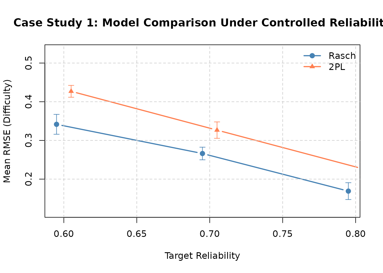

Grouped plot of difficulty RMSE by model and target reliability with error bars across replications.

Difficulty RMSE by model and target reliability. When reliability is controlled, the comparison isolates the effect of model structure on parameter recovery. Error bars show the range across replications.

Interpretation

With the calibration objective held constant, differences are no longer due to an intended reliability imbalance. They may still combine realized-form variation, response sampling, model structure, and the Rasch-oriented recovery estimator used here. The small executable run illustrates these patterns but does not estimate stable operating characteristics:

Higher reliability leads to smaller RMSE for both models, as expected. Better data quality (higher signal-to-noise ratio) improves parameter recovery.
Model differences are modest when reliability is held constant. Without reliability control, the 2PL model often appears to have worse difficulty recovery, but much of that apparent difference vanishes once reliability is equalized.
The critical role of controlling reliability: the differences within a model across reliability levels are typically larger than the differences between models at a fixed reliability level.

Methods text

We compared Rasch and 2PL item difficulty recovery under controlled reliability using the IRTsimrel R package (Lee, 2026). For each of six conditions (2 models x 3 target reliabilities: 0.60, 0.70, 0.80), item discriminations were calibrated to the target average-information reliability using EQC with M = 5{,}000 quadrature points. Tests comprised I = 20 items with normally distributed difficulties. For each condition, this executable demonstration used R = 5 replications of N = 300 simulees; production studies should increase both values. Item difficulties were estimated with a fast log-odds estimator and evaluated via bias and RMSE. We report the maximum calibration-quadrature residual across conditions separately from response-sample recovery error.

Case Study 2: Latent Distribution Robustness

Research question

How does latent distribution misspecification affect item parameter recovery when the test was calibrated for reliability under normality?

This study investigates what happens when data are generated from a distribution that differs from the one used during reliability calibration. In practice, test developers often assume normality when calibrating items, but the actual examinee population may be skewed, bimodal, or heavy-tailed.

Design

Component	Specification
Calibration shape	Normal
Generating shapes	Normal, skew_pos, bimodal, heavy_tail
Target reliability	0.80 (calibrated under normal)
Test length	20 items
N persons	300
Replications	5 (use 500+ in practice)

Key insight: When you calibrate under one distribution but generate under another, the achieved reliability will differ from the target because the test information profile interacts with the latent distribution.

Step 1: Calibrate under normal

cs2_calib <- eqc_calibrate(
  target_rho   = 0.80,
  n_items      = 20,
  model        = "rasch",
  latent_shape = "normal",
  item_source  = "parametric",
  reliability_metric = "info",
  M            = 5000L,
  seed         = 42,
  verbose      = FALSE
)

cat(sprintf("Calibrated c* = %.4f (under normal, rho = %.4f)\n",
            cs2_calib$c_star, cs2_calib$achieved_rho))
#> Calibrated c* = 1.0183 (under normal, rho = 0.8000)

gen_shapes <- c("normal", "skew_pos", "bimodal", "heavy_tail")
n_items   <- 20
n_persons <- 300
R <- 5

Step 2: Estimate reliability under each generating distribution

Before running the response simulation, we can estimate reliability under each generating distribution using the calibrated item parameters. This uses compute_rho_tilde() with an independent Monte Carlo theta sample from each distribution. The result is a conditional empirical approximation, not an exact theoretical coefficient.

# Estimate reliability under each generating distribution
actual_rho <- numeric(length(gen_shapes))
names(actual_rho) <- gen_shapes

for (j in seq_along(gen_shapes)) {
  theta_check <- sim_latentG(n = 5000, shape = gen_shapes[j], seed = 42)$theta
  actual_rho[j] <- compute_rho_tilde(
    c         = cs2_calib$c_star,
    theta_vec = theta_check,
    beta_vec  = cs2_calib$beta_vec,
    lambda_base = cs2_calib$lambda_base,
    theta_var = var(theta_check)
  )
}

rho_table <- data.frame(
  gen_shape    = gen_shapes,
  target_rho   = 0.80,
  actual_rho   = round(actual_rho, 4),
  rho_shift    = round(actual_rho - 0.80, 4)
)
cat("Independent-grid reliability estimate under each distribution:\n")
#> Independent-grid reliability estimate under each distribution:
print(rho_table)
#>             gen_shape target_rho actual_rho rho_shift
#> normal         normal        0.8     0.8000    0.0000
#> skew_pos     skew_pos        0.8     0.8004    0.0004
#> bimodal       bimodal        0.8     0.7962   -0.0038
#> heavy_tail heavy_tail        0.8     0.8001    0.0001

The reliability shifts when the generating distribution differs from the calibration distribution. This shift arises because the test information function \mathcal{J}(\theta; c^*) is not uniform across \theta, so different latent distributions weight the information differently.

Step 3: Run replications

cs2_results <- data.frame(
  gen_shape = character(), rep = integer(),
  bias_beta = numeric(), rmse_beta = numeric(),
  mean_p = numeric(),
  stringsAsFactors = FALSE
)

for (j in seq_along(gen_shapes)) {
  for (r in seq_len(R)) {
    sim <- simulate_response_data(
      result       = cs2_calib,
      n_persons    = n_persons,
      latent_shape = gen_shapes[j],
      seed         = 2000 * j + r
    )

    beta_true <- sim$beta
    p_items   <- colMeans(sim$response_matrix)
    p_items   <- pmin(pmax(p_items, 0.001), 0.999)
    beta_hat  <- -log(p_items / (1 - p_items))
    beta_hat  <- beta_hat - mean(beta_hat)

    bias <- mean(beta_hat - beta_true)
    rmse <- sqrt(mean((beta_hat - beta_true)^2))

    cs2_results <- rbind(cs2_results, data.frame(
      gen_shape = gen_shapes[j], rep = r,
      bias_beta = bias, rmse_beta = rmse,
      mean_p = mean(colMeans(sim$response_matrix)),
      stringsAsFactors = FALSE
    ))
  }
}

Results

cs2_summary <- aggregate(
  cbind(bias_beta, rmse_beta, mean_p) ~ gen_shape,
  data = cs2_results,
  FUN = function(x) round(mean(x), 4)
)
names(cs2_summary)[2:4] <- c("mean_bias", "mean_RMSE", "mean_prop_correct")

# Add actual reliability
cs2_summary$actual_rho <- round(actual_rho[cs2_summary$gen_shape], 4)
cs2_summary$rho_shift  <- round(actual_rho[cs2_summary$gen_shape] - 0.80, 4)

# Reorder columns for clarity
cs2_summary <- cs2_summary[, c("gen_shape", "actual_rho", "rho_shift",
                                 "mean_bias", "mean_RMSE", "mean_prop_correct")]

cat("Case Study 2: Latent Distribution Robustness Results\n")
#> Case Study 2: Latent Distribution Robustness Results
cat("====================================================\n")
#> ====================================================
print(cs2_summary)
#>    gen_shape actual_rho rho_shift mean_bias mean_RMSE mean_prop_correct
#> 1    bimodal     0.7962   -0.0038         0    0.1493            0.5019
#> 2 heavy_tail     0.8001    0.0001         0    0.1481            0.4934
#> 3     normal     0.8000    0.0000         0    0.1756            0.5025
#> 4   skew_pos     0.8004    0.0004         0    0.1411            0.4867

oldpar <- par(mfrow = c(2, 1), mar = c(4, 4, 3, 1))

# Panel 1: Reliability shift
bar_colors <- c("steelblue", "coral", "seagreen", "orchid")
bp <- barplot(actual_rho, col = bar_colors,
              ylim = c(0.5, 1.0), ylab = "Achieved Reliability",
              main = "Independent-Grid Reliability Estimate",
              names.arg = gen_shapes, las = 1, cex.names = 0.8)
abline(h = 0.80, col = "red", lty = 2, lwd = 2)
text(bp[1], 0.82, "Target = 0.80", col = "red", adj = 0, cex = 0.8)

# Add value labels
text(bp, actual_rho + 0.02, labels = round(actual_rho, 3), cex = 0.8)

# Panel 2: RMSE
rmse_vals <- cs2_summary$mean_RMSE
names(rmse_vals) <- cs2_summary$gen_shape
bp2 <- barplot(rmse_vals, col = bar_colors,
               ylab = "Mean RMSE (Difficulty)",
               main = "Difficulty RMSE by Generating Distribution",
               las = 1, cex.names = 0.8)

# Add value labels
text(bp2, rmse_vals + max(rmse_vals) * 0.03,
     labels = round(rmse_vals, 3), cex = 0.8)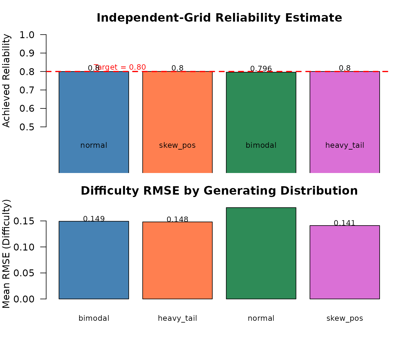

Two-panel bar plot showing estimated reliability and difficulty RMSE by generating latent shape.

Impact of latent distribution misspecification. Top: independent-grid reliability estimates shift away from the 0.80 target under non-normal generation. Bottom: difficulty RMSE varies with generating shape.


par(oldpar)

Interpretation

When the generating distribution does not match the calibration distribution, two things happen:

Reliability shifts: the independent-grid estimate deviates from the target (sometimes higher, sometimes lower), depending on how the test information profile aligns with the new distribution.
Recovery accuracy changes: RMSE is partly driven by the reliability shift and partly by the distribution’s effect on the information profile at each ability level.

Key findings:

Normal (matched condition): reliability is at the target, and RMSE serves as the baseline.
Positively skewed: more examinees are located in the left tail where item information may be lower for items centered near \beta = 0.
Bimodal: two modes create regions of low density near \theta = 0 where most items provide maximal information, potentially reducing effective information utilization.
Heavy-tailed: extreme ability values fall in regions of very low item information and can reduce average information for this fixed form.

This demonstrates why it is critical to either (a) calibrate under the intended generating distribution, or (b) report an independently evaluated reliability estimate under the generating distribution when intentionally mismatching.

Methods text

To assess robustness to latent distribution misspecification, we calibrated item parameters to \tilde{\rho}^* = 0.80 under a normal latent distribution using EQC (M = 5{,}000; I = 20 Rasch items). Response data were then generated under four distributions: normal, positively skewed (Gamma, k = 4), bimodal (\delta = 0.8), and heavy-tailed (Student-t, df = 5), all pre-standardized to mean 0 and variance 1. This executable demonstration used R = 5 replications of N = 300 simulees per condition; a production study should set replication count from a Monte Carlo precision target. We report both an independent Monte Carlo average-information estimate under each generating distribution and the difficulty recovery RMSE.

Case Study 3: Sample Size Planning

Research question

What minimum sample size is needed for stable item difficulty recovery at \tilde{\rho} = 0.80?

This study varies sample size while holding all other factors constant, producing an RMSE-vs-N curve that identifies the point of diminishing returns. This is a fundamental practical question: how many examinees are needed to achieve adequate parameter recovery?

Design

Factor	Specification
Sample size	50, 100, 200, 500
Model	Rasch
Reliability	0.80
Test length	20 items
Replications	5 (use 500+ in practice)

Step 1: Calibrate once

Since reliability and all other factors are held constant, we calibrate only once. The same calibrated parameters are used for all sample sizes.

cs3_calib <- eqc_calibrate(
  target_rho   = 0.80,
  n_items      = 20,
  model        = "rasch",
  item_source  = "parametric",
  reliability_metric = "info",
  M            = 5000L,
  seed         = 42,
  verbose      = FALSE
)

cat(sprintf("Calibrated c* = %.4f, achieved rho = %.4f\n",
            cs3_calib$c_star, cs3_calib$achieved_rho))
#> Calibrated c* = 1.0183, achieved rho = 0.8000

sample_sizes <- c(50, 100, 200, 500)
R <- 5

Step 2: Run replications

cs3_results <- data.frame(
  n_persons = integer(), rep = integer(),
  rmse_beta = numeric(), bias_beta = numeric(),
  max_abs_err = numeric(),
  stringsAsFactors = FALSE
)

for (n_idx in seq_along(sample_sizes)) {
  N <- sample_sizes[n_idx]

  for (r in seq_len(R)) {
    sim <- simulate_response_data(
      result    = cs3_calib,
      n_persons = N,
      seed      = 3000 * n_idx + r
    )

    beta_true <- sim$beta
    p_items   <- colMeans(sim$response_matrix)
    p_items   <- pmin(pmax(p_items, 0.001), 0.999)
    beta_hat  <- -log(p_items / (1 - p_items))
    beta_hat  <- beta_hat - mean(beta_hat)

    bias     <- mean(beta_hat - beta_true)
    rmse     <- sqrt(mean((beta_hat - beta_true)^2))
    max_abs  <- max(abs(beta_hat - beta_true))

    cs3_results <- rbind(cs3_results, data.frame(
      n_persons = N, rep = r,
      rmse_beta = rmse, bias_beta = bias,
      max_abs_err = max_abs,
      stringsAsFactors = FALSE
    ))
  }
}

Results

cs3_summary <- aggregate(
  cbind(bias_beta, rmse_beta, max_abs_err) ~ n_persons,
  data = cs3_results,
  FUN = function(x) round(mean(x), 4)
)
names(cs3_summary)[2:4] <- c("mean_bias", "mean_RMSE", "mean_max_err")

# Add SD of RMSE across reps
cs3_rmse_sd <- aggregate(rmse_beta ~ n_persons, data = cs3_results, FUN = sd)
cs3_summary$sd_RMSE <- round(cs3_rmse_sd$rmse_beta, 4)

cat("Case Study 3: Sample Size Planning Results\n")
#> Case Study 3: Sample Size Planning Results
cat("============================================\n")
#> ============================================
print(cs3_summary)
#>   n_persons mean_bias mean_RMSE mean_max_err sd_RMSE
#> 1        50         0    0.2843       0.5970  0.0283
#> 2       100         0    0.1867       0.4264  0.0194
#> 3       200         0    0.1906       0.4914  0.0208
#> 4       500         0    0.1315       0.3336  0.0277

# Prepare data
N_vals <- cs3_summary$n_persons
rmse_mean <- cs3_summary$mean_RMSE
rmse_sd   <- cs3_summary$sd_RMSE

# Plot
plot(N_vals, rmse_mean,
     type = "b", pch = 19, col = "steelblue", lwd = 2,
     xlab = "Sample Size (N)", ylab = "Mean RMSE (Difficulty)",
     main = "Case Study 3: RMSE vs. Sample Size at Fixed Reliability",
     log = "x", ylim = c(0, max(rmse_mean + rmse_sd) * 1.2))

# Shaded confidence region
polygon(
  c(N_vals, rev(N_vals)),
  c(rmse_mean - rmse_sd, rev(rmse_mean + rmse_sd)),
  col = adjustcolor("steelblue", alpha.f = 0.2), border = NA
)

# Re-draw line on top
lines(N_vals, rmse_mean, type = "b", pch = 19, col = "steelblue", lwd = 2)

# Add reference line at N = 200
abline(v = 200, col = "red", lty = 3)
text(200, max(rmse_mean) * 0.95, "N = 200", col = "red", pos = 4, cex = 0.8)

# Add value labels
text(N_vals, rmse_mean + rmse_sd + max(rmse_mean) * 0.05,
     labels = round(rmse_mean, 3), cex = 0.8)

grid(lty = 2, col = "gray80")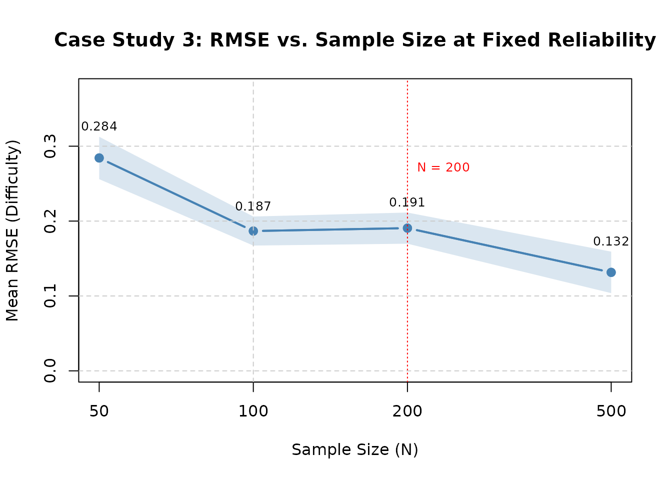

Line plot showing difficulty RMSE decreasing as sample size increases with a shaded variability band.

Difficulty RMSE as a function of sample size at fixed reliability (rho = 0.80). RMSE decreases monotonically with N. The shaded region shows plus/minus one standard deviation across replications.

RMSE scaling analysis

Theoretical prediction: under regularity conditions, RMSE should scale approximately as O(1/\sqrt{N}). We can check this by examining the ratio of RMSE values:

# Check the O(1/sqrt(N)) scaling
cat("Theoretical RMSE scaling check:\n")
#> Theoretical RMSE scaling check:
cat("If RMSE ~ 1/sqrt(N), then RMSE * sqrt(N) should be constant.\n\n")
#> If RMSE ~ 1/sqrt(N), then RMSE * sqrt(N) should be constant.

cs3_summary$rmse_x_sqrtN <- round(cs3_summary$mean_RMSE * sqrt(cs3_summary$n_persons), 4)
print(cs3_summary[, c("n_persons", "mean_RMSE", "rmse_x_sqrtN")])
#>   n_persons mean_RMSE rmse_x_sqrtN
#> 1        50    0.2843       2.0103
#> 2       100    0.1867       1.8670
#> 3       200    0.1906       2.6955
#> 4       500    0.1315       2.9404

If the product RMSE \times \sqrt{N} is approximately constant across sample sizes, it confirms the expected O(1/\sqrt{N}) scaling.

Practical interpretation

The five-replication run is a rendering-friendly pilot, not a basis for a universal minimum sample size. Use its curve to define a candidate range, then increase replications and attach Monte Carlo uncertainty to the RMSE criterion. The required N is specific to the estimator, item form, reliability metric, latent distribution, and tolerance. Different reliability levels can shift the curve, so they should be crossed explicitly rather than extrapolated from this one condition.

Methods text

To determine the minimum sample size for stable item difficulty recovery, we calibrated a 20-item Rasch test to \tilde{\rho}^* = 0.80 using EQC. Response data were generated for N \in \{50, 100, 200, 500\} simulees across R = 5 demonstration replications per condition. Item difficulties were estimated with a fast log-odds estimator and evaluated by RMSE. The pilot RMSE curve was used to identify candidate sample sizes for a larger, precision-calibrated replication study; it was not treated as a definitive minimum-N rule.

Adapt for Your Study

The three case studies above are templates. To adapt them for your research, follow the planning and reporting checklists below.

Planning checklist

Before running your study, verify the following:

Define the research question clearly and precisely. The question should specify what comparison is being made and what metrics will be used to evaluate it.
Select the IRT model(s) appropriate for your context. Use "rasch" for tests with equal discriminations, "2pl" for tests with varying discriminations, and "3pl" when lower asymptotes are part of the DGP. For 3PL, specify and report guessing_params and the package’s D = 1 logistic convention.
Choose the latent distribution(s) that represent your target population. Use "normal" as a baseline and add non-normal shapes to test robustness.
Set target reliability levels that span the range relevant to your application. Include at least three levels to detect nonlinear effects.
Screen all design cells for feasibility using check_feasibility(). Remove or modify any infeasible cells.
Determine the number of replications from the desired Monte Carlo standard error or confidence-interval width. Small values are suitable only for code pilots; there is no universal publication threshold.
Establish a seed management scheme for complete reproducibility. Record all seeds in your analysis script.

Template code

The following template can be adapted for any simulation study using IRTsimrel. Replace the bracketed comments with your study’s parameters.

# =============================================================
# IRTsimrel Simulation Study Template
# =============================================================
#
# Research Question:
#   [State your research question here]
#
# Author: JoonHo Lee (jlee296@ua.edu)
# Date:   2026-07-01
# =============================================================

library(IRTsimrel)

# ---- 1. Design ----
design <- expand.grid(
  target_rho   = c(0.60, 0.70, 0.80),      # [your reliability levels]
  n_items      = c(20, 40),                  # [your test lengths]
  model        = c("rasch", "2pl"),          # add "3pl" plus item_params when needed
  latent_shape = c("normal", "skew_pos"),    # [your latent shapes]
  stringsAsFactors = FALSE
)

N_PERSONS  <- 1000     # [your sample size]
R          <- 500      # [your replications]
M_QUAD     <- 10000L   # [your quadrature size]
CALIB_SEED <- 42       # [your calibration seed]

# ---- 2. Feasibility screening ----
design$feasible <- NA
for (i in seq_len(nrow(design))) {
  feas <- check_feasibility(
    n_items      = design$n_items[i],
    model        = design$model[i],
    latent_shape = design$latent_shape[i],
    item_source  = "parametric",
    target_rho   = design$target_rho[i],
    M            = M_QUAD,
    seed         = CALIB_SEED,
    verbose      = FALSE
  )
  design$feasible[i] <-
    identical(feas$target_status_info_canonical, "feasible") &&
    feas$admissible_root_count_info > 0L
}
design <- design[design$feasible, ]
cat(sprintf("Feasible cells: %d\n", nrow(design)))

# ---- 3. Calibration ----
calib_list <- vector("list", nrow(design))
for (i in seq_len(nrow(design))) {
  d <- design[i, ]
  calib_list[[i]] <- eqc_calibrate(
    target_rho   = d$target_rho,
    n_items      = d$n_items,
    model        = d$model,
    latent_shape = d$latent_shape,
    item_source  = "parametric",
    reliability_metric = "info",
    M            = M_QUAD,
    seed         = CALIB_SEED,
    verbose      = FALSE
  )
}

# ---- 4. Verification ----
design$achieved_rho <- vapply(calib_list,
  function(r) r$achieved_rho, numeric(1))
design$abs_error <- abs(design$achieved_rho - design$target_rho)
cat(sprintf("Max calibration error: %.2e\n", max(design$abs_error)))

# ---- 5. Simulation loop ----
output <- data.frame()

for (i in seq_len(nrow(design))) {
  d <- design[i, ]

  for (r in seq_len(R)) {
    sim <- simulate_response_data(
      result       = calib_list[[i]],
      n_persons    = N_PERSONS,
      latent_shape = d$latent_shape,
      seed         = 1000 * i + r
    )
    sim_provenance <- sim$provenance[c("metric", "calibration_status",
                                       "status_flags", "item_source",
                                       "simulation_seed", "latent_shape")]

    # ---- Your analysis here ----
    beta_true <- sim$beta
    p_items <- colMeans(sim$response_matrix)
    p_items <- pmin(pmax(p_items, 0.001), 0.999)
    beta_hat <- -log(p_items / (1 - p_items))
    beta_hat <- beta_hat - mean(beta_hat)
    rmse <- sqrt(mean((beta_hat - beta_true)^2))
    bias <- mean(beta_hat - beta_true)

    output <- rbind(output, data.frame(
      cell = i, rep = r,
      target_rho = d$target_rho, model = d$model,
      n_items = d$n_items, latent_shape = d$latent_shape,
      rmse = rmse, bias = bias,
      metric = sim_provenance$metric,
      calibration_status = sim_provenance$calibration_status,
      simulation_seed = sim_provenance$simulation_seed
    ))
  }
}

# ---- 6. Summarize ----
summary_table <- aggregate(
  cbind(rmse, bias) ~ target_rho + model + n_items + latent_shape,
  data = output, FUN = mean
)
print(summary_table)

Reporting checklist

When writing up your simulation study, include the following:

State IRTsimrel version and cite Lee (2026).
Specify the calibration algorithm (EQC or SAC) and its parameters.
Report the reliability metric (average-information or MSEM-based).
List all target reliability levels.
Describe item parameter source and generation method.
State latent distribution(s) and shape parameters.
Report feasibility screening results (number screened, number infeasible).
Report root policy, selected-root status, item scope, and maximum calibration-quadrature residual across all cells.
State the number of replications and persons per replication.
Describe seed management for reproducibility.
For 3PL, report lower-asymptote generation and the D = 1 convention.
Distinguish calibration, independent holdout, and response-estimator reliability evidence.

Summary and Recommendations

The three case studies illustrate the following general principles:

Principle 1: Always control reliability. Without it, model comparisons are confounded by data quality differences. Case Study 1 demonstrates how reliability control isolates the effect of model structure on parameter recovery. The differences within a model across reliability levels are often larger than the differences between models at a fixed reliability.

Principle 2: Document distribution mismatches. If the calibration and generating distributions differ, report the actual achieved reliability under the generating distribution. Case Study 2 shows that misspecification shifts both reliability and recovery accuracy in predictable but important ways.

Principle 3: Use RMSE curves for sample size planning. A reliability-controlled RMSE-vs-N curve provides an objective basis for choosing sample size. Case Study 3 demonstrates diminishing returns beyond a minimum threshold and confirms the theoretical O(1/\sqrt{N}) scaling.

Principle 4: Start with feasibility screening. Before committing to a large simulation, use check_feasibility() and rho_curve() to verify that your design is achievable. Infeasible cells waste computational resources and produce misleading boundary solutions.

Principle 5: Report thoroughly. Follow the reporting checklist and include a methods paragraph based on the templates provided. Transparent reporting enables replication and builds confidence in your findings.

For additional background, see:

vignette("introduction") – package overview.
vignette("simulation-design") – factorial design framework.
vignette("algorithm-eqc") – Algorithm 1 details.
vignette("algorithm-sac") – Algorithm 2 (SAC) for validation.
vignette("validation") – TAM-based validation procedures.

References

Lee, J.-H. (2026). Reliability-Targeted Simulation of Item Response Data: Solving the Inverse Design Problem. arXiv:2512.16012v2. https://doi.org/10.48550/arXiv.2512.16012

Robbins, H., & Monro, S. (1951). A stochastic approximation method. The Annals of Mathematical Statistics, 22(3), 400–407.

JoonHo Lee (jlee296@ua.edu)

2026-08-22

Overview

Case Study 1: Model Comparison Under Controlled Reliability

Research question

Design

Step 1: Feasibility screening

Step 2: Calibrate all conditions

Step 3: Run replications

Results

Interpretation

Methods text

Case Study 2: Latent Distribution Robustness

Research question

Design

Step 1: Calibrate under normal

Step 2: Estimate reliability under each generating distribution

Step 3: Run replications

Results

Interpretation

Methods text

Case Study 3: Sample Size Planning

Research question

Design

Step 1: Calibrate once

Step 2: Run replications

Results

RMSE scaling analysis

Practical interpretation

Methods text

Adapt for Your Study

Planning checklist

Template code

Reporting checklist

Summary and Recommendations

References