IRTsimrel

IRTsimrel provides a principled framework for reliability-targeted simulation of Item Response Theory (IRT) data. Instead of treating reliability as an implicit outcome of simulation design choices, IRTsimrel allows researchers to specify a target reliability level as an explicit input parameter.

The Problem

In Monte Carlo simulation studies for IRT, researchers routinely vary sample size, test length, and item parameters—but marginal reliability is almost never directly controlled. This creates:

Ecological validity threats: Real assessments often have reliabilities of 0.5–0.7, but simulations may implicitly assume higher values
Confounded comparisons: Conclusions about model superiority may only hold within certain reliability regimes
Limited replicability: Without knowing implied reliability, exact replication is impossible

The Solution: Think Like Multilevel Modelers

In multilevel modeling, the intraclass correlation (ICC) is always a primary design factor. ICC determines the signal-to-noise ratio—the proportion of variance at the cluster level versus residual level.

Marginal reliability in IRT serves the same role as ICC in multilevel models.

IRTsimrel brings IRT simulation methodology into alignment with this best practice.

Installation

You can install the development version of IRTsimrel from GitHub with:

# install.packages("pak")
pak::pak("joonho112/IRTsimrel")

Quick Start

Suppose you want to simulate Rasch model data with:

25 items
Target reliability of 0.80
Normal latent trait distribution

Step 1: Calibrate

library(IRTsimrel)

# Calibrate to achieve target reliability
eqc_result <- eqc_calibrate(
  target_rho = 0.80,
  n_items = 25,
  model = "rasch",
  latent_shape = "normal",
  item_source = "parametric",
  M = 10000,
  seed = 42
)

eqc_result
#> 
#> =======================================================
#>   Empirical Quadrature Calibration (EQC) Results
#> =======================================================
#> 
#> Calibration Summary:
#>   Model                        : RASCH
#>   Target reliability (rho*)    : 0.8000
#>   Achieved reliability         : 0.8000
#>   Absolute error               : 3.77e-06
#>   Scaling factor (c*)          : 0.9277
#> 
#> Design Parameters:
#>   Number of items (I)          : 25
#>   Quadrature points (M)        : 10000
#>   Reliability metric           : MSEM-based (bar/w)
#>   Latent variance              : 1.0123
#> 
#> Convergence:
#>   Root status                  : uniroot_success
#>   Search bracket               : [0.300, 3.000]
#>   Bracket reliabilities        : [0.3538, 0.9020]
#> 
#> Parameter Summaries:
#>   theta:        mean = -0.011, sd = 1.006
#>   beta:         mean = -0.000, sd = 0.909, range = [-1.60, 1.73]
#>   lambda_base:  mean = 1.000, sd = 0.000
#>   lambda_scaled: mean = 0.928, sd = 0.000

Step 2: Generate Data

# Generate response data with calibrated parameters
sim_data <- simulate_response_data(
  eqc_result = eqc_result,
  n_persons = 1000,
  latent_shape = "normal",
  seed = 123
)

# Response matrix ready for analysis
dim(sim_data$response_matrix)
#> [1] 1000   25

Step 3: Validate (Optional)

# Validate with TAM package
tam_rel <- compute_reliability_tam(
  resp = sim_data$response_matrix,
  model = "rasch"
)

cat(sprintf("Target:  %.3f\n", 0.80))
cat(sprintf("WLE:     %.3f\n", tam_rel$rel_wle))
cat(sprintf("EAP:     %.3f\n", tam_rel$rel_eap))

Key Features

Two Calibration Algorithms

Algorithm	Function	Best For
EQC (Empirical Quadrature Calibration)	`eqc_calibrate()`	Routine use, fast & accurate
SPC (Stochastic Approximation Calibration)	`spc_calibrate()`	Validation, complex DGPs

Flexible Latent Distributions

compare_shapes(
  n = 3000,
  shapes = c("normal", "bimodal", "skew_pos", "heavy_tail"),
  seed = 42
)

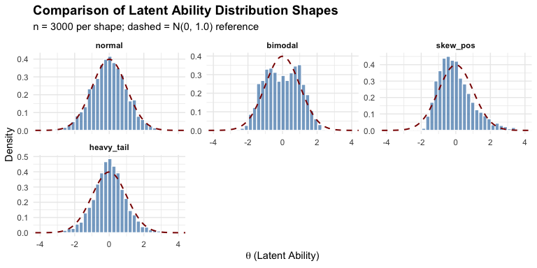
12 built-in shapes including normal, bimodal, trimodal, skewed, heavy-tailed, uniform, and floor/ceiling effects—all pre-standardized to mean 0 and variance 1.

Realistic Item Parameters

Generate item parameters with empirically-grounded characteristics:

# IRW-based difficulties with copula-correlated discriminations
items <- sim_item_params(
  n_items = 30,
  model = "2pl",
  source = "irw",
  method = "copula",
  discrimination_params = list(rho = -0.3)  # Empirical correlation
)

The Core Principle: Separation of Structure and Scale

IRTsimrel implements a fundamental principle:

Structure: Realistic item characteristics and flexible latent distributions come from empirically-grounded generators
Scale: A global discrimination scaling factor $c^*$ is calibrated to achieve target reliability

$\lambda_i^* = c^* \cdot \lambda_{i,0}$

This allows researchers to study the effect of reliability on estimation while maintaining realistic data structures.

Two Reliability Metrics

Metric	Formula	Used By
MSEM-based ( $\bar{\rho}$ )	$\frac{\sigma^2_\theta}{\sigma^2_\theta + E[1/\mathcal{J}(\theta)]}$	SPC (theoretically exact)
Average-information ( $\tilde{\rho}$ )	$\frac{\sigma^2_\theta \bar{\mathcal{J}}}{\sigma^2_\theta \bar{\mathcal{J}} + 1}$	EQC (faster)

By Jensen’s inequality: $\tilde{\rho} \geq \bar{\rho}$ always holds.

Vignettes

For detailed guidance, see the package vignettes:

vignette("introduction_to_irtsimrel") — Package overview and workflow
vignette("latent_distributions") — Working with 12 latent shapes
vignette("item_parameters") — Generating realistic item parameters
vignette("eqc_algorithm") — Algorithm 1: EQC details
vignette("spc_algorithm") — Algorithm 2: SPC details
vignette("validation") — Validating calibration results

Citation

If you use IRTsimrel in your research, please cite:

Lee, J.-H. (2025). Reliability-targeted simulation for item response data.
arXiv preprint. arXiv:XXXX.XXXXX

TAM — Test Analysis Modules for IRT
mirt — Multidimensional Item Response Theory
irw — Item Response Warehouse