Designing IRT Simulation Studies with Reliability Control

Overview

Reading time: approximately 25–30 minutes.

This vignette shows how to use IRTsimrel to design rigorous, reproducible IRT simulation studies with reliability as an explicit design factor. By the end of this vignette you will be able to:

Articulate why marginal reliability must be controlled in simulation designs.
Set up a complete factorial design that crosses reliability with other factors.
Screen all cells for feasibility before committing to calibration.
Visualize reliability curves across design conditions.
Execute batch calibration and batch data generation across all cells.
Verify calibration residuals in every cell and distinguish them from independent holdout or response-estimator evidence.
Apply recommended practices for seed management, reporting, and parallelization.

Prerequisites: familiarity with eqc_calibrate() and the basics of IRT simulation. See vignette("introduction") for background.

Why Reliability Should Be a Design Factor

The ICC analogy

In multilevel modeling (MLM), no competent simulation study would omit the intraclass correlation (ICC) from its factorial design. The ICC determines the signal-to-noise ratio at the cluster level, and every methodological conclusion is conditioned on that ratio. Studying a new estimator only at ICC = 0.10 tells us nothing about how it performs at ICC = 0.30.

Marginal reliability plays exactly the same role in IRT. It captures the proportion of latent variance that is “signal” versus “noise,” and it governs the precision of every person-parameter estimate. Yet in the vast majority of published IRT simulation studies, reliability is neither controlled nor even reported.

The analogy is precise:

MLM simulation	IRT simulation
ICC is a primary design factor	Reliability should be a design factor
ICC controls cluster-level signal	Reliability controls person-level signal
Conclusions depend on ICC level	Conclusions depend on reliability level
Always reported in Methods section	Rarely reported in Methods section

What happens without reliability control

When reliability is not controlled, several problems arise:

Confounded comparisons: two models may appear to differ not because of their structural properties but because they operate at different reliability levels. The “winning” model may simply have been handed better data.
Limited generalizability: results obtained at an unknown reliability (implicitly determined by item parameter choices) do not generalize to other reliability regimes.
Irreproducibility: without knowing the implied reliability, another researcher cannot replicate the exact simulation conditions.
Ecological invalidity: real-world assessments span a wide range of reliabilities (0.50 to 0.95). A simulation that only explores one unknown reliability point misses most of this range.

A cautionary tale

Consider a researcher who wants to compare the Rasch model and the 2PL model in terms of item-difficulty recovery. A naive design might fix 20 items, normal abilities, and 500 persons, then generate one Rasch data set and one 2PL data set. The researcher finds that RMSE is substantially larger under the 2PL model and concludes the Rasch model recovers difficulty better.

The problem: the two data sets may have very different reliabilities. If the 2PL data happen to have lower reliability (because of how discriminations were drawn), then higher RMSE is an artifact of the noisier data, not a property of the generating model. The conclusion is confounded.

With IRTsimrel, the researcher can hold reliability constant across both models. Any remaining difference in RMSE is then attributable to model structure, not data quality.

# Calibrate Rasch and 2PL to the SAME reliability
eqc_rasch <- eqc_calibrate(
  target_rho = 0.80, n_items = 20, model = "rasch",
  item_source = "parametric", reliability_metric = "info",
  M = 5000L, seed = 42
)

eqc_2pl <- eqc_calibrate(
  target_rho = 0.80, n_items = 20, model = "2pl",
  item_source = "parametric", reliability_metric = "info",
  M = 5000L, seed = 42
)

cat(sprintf("Rasch achieved rho: %.4f  (c* = %.4f)\n",
            eqc_rasch$achieved_rho, eqc_rasch$c_star))
#> Rasch achieved rho: 0.8000  (c* = 1.0183)
cat(sprintf("2PL   achieved rho: %.4f  (c* = %.4f)\n",
            eqc_2pl$achieved_rho, eqc_2pl$c_star))
#> 2PL   achieved rho: 0.8000  (c* = 0.9026)

Both conditions now operate at the same marginal reliability. Any downstream difference in RMSE reflects the structural difference between Rasch and 2PL, not an accidental reliability imbalance.

Reliability as an experimental control

Controlling reliability in IRT simulation is analogous to controlling temperature in a chemistry experiment. You would never compare two reactions at different temperatures and attribute the difference solely to the reagents. Similarly, comparing two IRT models at different reliabilities conflates model structure with data quality.

IRTsimrel enables this control by solving the inverse design problem: given a target reliability \rho^*, find the global discrimination scaling factor c^* such that a selected empirical reliability objective matches \rho^*. eqc_calibrate() maps the requested log-scale interval, then uses Brent polishing on detected local crossings and an explicit branch policy. Population agreement is assessed separately with larger or independent Monte Carlo draws.

The Factorial Design Framework

A well-designed simulation study crosses multiple factors to map out the operating characteristics of the method under study. A natural four-factor design for IRT research is:

Factor	Levels	Rationale
Reliability	0.60, 0.70, 0.80	Low, moderate, high data quality
Test length	15, 30	Short vs. long forms
Latent shape	normal, skew_pos	Standard vs. violated normality
Model	rasch, 2pl	Equal vs. varying discriminations

Building the design matrix

design <- expand.grid(
  reliability  = c(0.60, 0.70, 0.80),
  n_items      = c(15, 30),
  latent_shape = c("normal", "skew_pos"),
  model        = c("rasch", "2pl"),
  stringsAsFactors = FALSE
)

cat(sprintf("Total cells: %d\n", nrow(design)))
#> Total cells: 24
head(design, 8)
#>   reliability n_items latent_shape model
#> 1         0.6      15       normal rasch
#> 2         0.7      15       normal rasch
#> 3         0.8      15       normal rasch
#> 4         0.6      30       normal rasch
#> 5         0.7      30       normal rasch
#> 6         0.8      30       normal rasch
#> 7         0.6      15     skew_pos rasch
#> 8         0.7      15     skew_pos rasch

We have 24 design cells. Before calibrating any of them, we should verify that every cell is feasible—that the target reliability can actually be achieved with the given item and latent configuration.

Choosing factor levels

When selecting factor levels, consider these guidelines:

Reliability: include at least three levels spanning the range relevant to your research context. Educational testing typically ranges from 0.60 (formative assessments) to 0.90 (high-stakes tests).
Test length: include at least two lengths that bracket the typical range for your application domain. Short forms (10–15 items) and standard forms (25–40 items) are common.
Latent distributions: always include "normal" as a baseline. Add one or two non-normal shapes to test robustness. Good choices include "skew_pos" (selective admissions) and "bimodal" (heterogeneous populations).
Model: include "rasch" and "2pl" if your study involves that model comparison. Add "3pl" when a plausible lower asymptote is scientifically relevant, and report its guessing_params. The example below intentionally remains a Rasch-versus-2PL design.

Feasibility Screening

The check_feasibility() function computes the achievable reliability range for a given test design. We loop over every cell and record whether the target reliability falls within the range for the “info” metric (the default and recommended metric for EQC).

Feasibility screening should always precede calibration. It is fast (a fraction of a second per cell) and prevents wasted effort on infeasible conditions.

# Screen all cells
design$feasible <- NA
design$rho_max  <- NA
design$rho_min  <- NA

for (i in seq_len(nrow(design))) {
  feas <- check_feasibility(
    n_items      = design$n_items[i],
    model        = design$model[i],
    latent_shape = design$latent_shape[i],
    item_source  = "parametric",
    target_rho   = design$reliability[i],
    c_bounds     = c(0.1, 10),
    M            = 5000L,
    seed         = 42,
    verbose      = FALSE
  )
  design$rho_min[i]  <- feas$rho_range_info[1]
  design$rho_max[i]  <- feas$rho_range_info[2]
  design$feasible[i] <-
    identical(feas$target_status_info_canonical, "feasible") &&
    feas$admissible_root_count_info > 0L
}

# Display summary
cat(sprintf("Feasible cells  : %d / %d\n",
            sum(design$feasible), nrow(design)))
#> Feasible cells  : 24 / 24
cat(sprintf("Infeasible cells: %d\n", sum(!design$feasible)))
#> Infeasible cells: 0

# Show the infeasible cells if any
if (any(!design$feasible)) {
  cat("\nInfeasible cells:\n")
  print(design[!design$feasible, ])
}

# Create a compact summary by n_items x model
feas_summary <- aggregate(
  cbind(rho_min, rho_max) ~ n_items + model,
  data = design, FUN = function(x) round(mean(x), 3)
)
names(feas_summary)[3:4] <- c("avg_rho_min", "avg_rho_max")
print(feas_summary)
#>   n_items model avg_rho_min avg_rho_max
#> 1      15   2pl       0.042       0.978
#> 2      30   2pl       0.082       0.990
#> 3      15 rasch       0.036       0.977
#> 4      30 rasch       0.070       0.989

Interpreting feasibility results

The output shows the range [\rho_{\min}, \rho_{\max}] achievable for each cell. Key patterns to look for:

Short tests (e.g., 15 items) have a lower maximum achievable reliability than long tests, because fewer items provide less total information.
Rasch vs. 2PL: The 2PL model may have a slightly different achievable range because varying discriminations change the effective information.
Non-normal latent distributions: skewed or heavy-tailed distributions may shift the achievable range because test information depends on the ability distribution.

When cells are infeasible

If any cell is infeasible, you have several options:

Increase c_bounds[2] (allow stronger discrimination scaling).
Increase n_items for that cell.
Drop the reliability level from the design.
Accept the achievable maximum and note the deviation.

For the remaining sections we proceed with all feasible cells only.

Reliability Curves Across Conditions

Reliability curves show how \rho(c) varies with the scaling factor c. They help you understand the shape and range of achievable reliability for each design condition.

The rho_curve() function computes reliability at a grid of c values using Monte Carlo integration with the same quadrature approach used by eqc_calibrate(). This visualization serves three purposes:

Maps topology: crossings, saturation, or an interior maximum may be visible; do not assume the curve is globally monotone.
Shows the displayed finite-grid range: use the adaptive topology from check_feasibility() rather than the display grid to classify a target.
Identifies where calibration occurs: the horizontal position where the curve crosses the target reliability.

# Select four representative conditions
conditions <- list(
  list(n_items = 15, model = "rasch",  latent_shape = "normal",
       label = "15 items, Rasch, Normal"),
  list(n_items = 30, model = "rasch",  latent_shape = "normal",
       label = "30 items, Rasch, Normal"),
  list(n_items = 15, model = "2pl",    latent_shape = "normal",
       label = "15 items, 2PL, Normal"),
  list(n_items = 30, model = "rasch",  latent_shape = "skew_pos",
       label = "30 items, Rasch, Skew+")
)

c_grid <- seq(0.1, 5, length.out = 40)

oldpar <- par(mfrow = c(2, 2), mar = c(4, 4, 3, 1))

for (cond in conditions) {
  curve_data <- rho_curve(
    c_values     = c_grid,
    n_items      = cond$n_items,
    model        = cond$model,
    latent_shape = cond$latent_shape,
    item_source  = "parametric",
    metric       = "info",
    M            = 5000L,
    seed         = 42,
    plot         = FALSE
  )

  plot(curve_data$c, curve_data$rho_tilde, type = "l", lwd = 2,
       col = "steelblue", ylim = c(0, 1),
       xlab = "Scaling factor c", ylab = expression(tilde(rho)),
       main = cond$label, cex.main = 0.9)
  abline(h = 0.70, col = "red", lty = 2)
  abline(h = 0.80, col = "red", lty = 3)
}

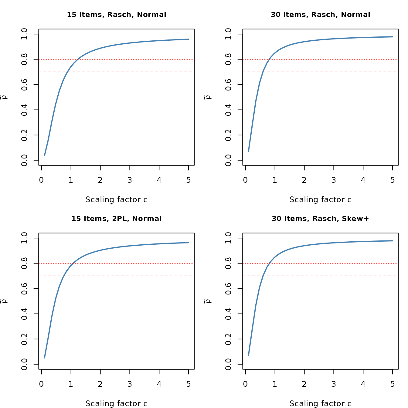
Four reliability curves comparing design conditions with dashed target reliability reference lines.

Reliability curves for four design conditions. Dashed red lines mark target reliabilities of 0.70 and 0.80. Differences in curve shape reflect how test length and latent distribution affect the reliability-discrimination relationship.


par(oldpar)

Key observations from the reliability curves:

Longer tests reach the same reliability with a smaller scaling factor c. For example, 30 items might achieve \tilde{\rho} = 0.80 at c \approx 1.2, whereas 15 items might require c \approx 2.0.
The 2PL model reaches high reliability faster because varying discriminations contribute additional information per item on average.
Skewed latent distributions shift the curve slightly, because test information concentrates where items are most informative. If the latent distribution places more mass in regions of lower information, the reliability curve is lower.
These representative Rasch/2PL curves rise over the displayed grid. That is an observation about these draws and bounds, not a global theorem. EQC still scans the full requested interval and polishes each detected crossing locally.

Batch Calibration

With the design validated, we calibrate every feasible cell. The code below stores results in a list indexed by cell number.

The key principle: calibrate once, generate many times. The calibrated parameters (item difficulties, scaled discriminations, and the quadrature sample) are fixed for a given cell. Multiple replications vary only the person sample.

# Keep only feasible cells
design_feasible <- design[design$feasible, ]

# Storage
results_list <- vector("list", nrow(design_feasible))

for (i in seq_len(nrow(design_feasible))) {
  d <- design_feasible[i, ]

  res <- eqc_calibrate(
    target_rho   = d$reliability,
    n_items      = d$n_items,
    model        = d$model,
    latent_shape = d$latent_shape,
    item_source  = "parametric",
    reliability_metric = "info",
    M            = 5000L,
    seed         = 42,
    verbose      = FALSE
  )

  results_list[[i]] <- res
}

# Attach achieved reliability to the design frame
design_feasible$achieved_rho <- vapply(
  results_list, function(r) r$achieved_rho, numeric(1)
)
design_feasible$c_star <- vapply(
  results_list, function(r) r$c_star, numeric(1)
)
design_feasible$abs_error <- abs(
  design_feasible$achieved_rho - design_feasible$reliability
)

cat(sprintf("Mean absolute error: %.6f\n", mean(design_feasible$abs_error)))
#> Mean absolute error: 0.000000
cat(sprintf("Max  absolute error: %.6f\n", max(design_feasible$abs_error)))
#> Max  absolute error: 0.000000

These residuals describe the fixed calibration quadrature. They can be much smaller than the Monte Carlo discrepancy on an independent theta draw; use a holdout evaluation when making population-level accuracy claims.

Examining the calibrated scaling factors

The calibrated c^* values reveal how much discrimination scaling is needed to reach each target reliability:

# Show c* by condition
cstar_table <- design_feasible[, c("model", "n_items", "latent_shape",
                                    "reliability", "c_star")]
cstar_table$c_star <- round(cstar_table$c_star, 4)
print(cstar_table)
#>    model n_items latent_shape reliability c_star
#> 1  rasch      15       normal         0.6 0.6789
#> 2  rasch      15       normal         0.7 0.8793
#> 3  rasch      15       normal         0.8 1.2342
#> 4  rasch      30       normal         0.6 0.4632
#> 5  rasch      30       normal         0.7 0.5900
#> 6  rasch      30       normal         0.8 0.8042
#> 7  rasch      15     skew_pos         0.6 0.7078
#> 8  rasch      15     skew_pos         0.7 0.9342
#> 9  rasch      15     skew_pos         0.8 1.3542
#> 10 rasch      30     skew_pos         0.6 0.4654
#> 11 rasch      30     skew_pos         0.7 0.5933
#> 12 rasch      30     skew_pos         0.8 0.8090
#> 13   2pl      15       normal         0.6 0.5791
#> 14   2pl      15       normal         0.7 0.7555
#> 15   2pl      15       normal         0.8 1.0716
#> 16   2pl      30       normal         0.6 0.4237
#> 17   2pl      30       normal         0.7 0.5417
#> 18   2pl      30       normal         0.8 0.7425
#> 19   2pl      15     skew_pos         0.6 0.7357
#> 20   2pl      15     skew_pos         0.7 0.9678
#> 21   2pl      15     skew_pos         0.8 1.3950
#> 22   2pl      30     skew_pos         0.6 0.4347
#> 23   2pl      30     skew_pos         0.7 0.5550
#> 24   2pl      30     skew_pos         0.8 0.7580

Note that c^* > 1 means the baseline discriminations were scaled up (items made more discriminating), while c^* < 1 means they were scaled down. Higher target reliability generally requires a larger c^*, and longer tests require a smaller c^* for the same target.

Batch Data Generation

After calibration, we generate response data for each cell. In a real study you would embed this in a replication loop; here we generate a single data set per cell for illustration.

sim_data_list <- vector("list", nrow(design_feasible))

for (i in seq_len(nrow(design_feasible))) {
  d <- design_feasible[i, ]

  sim_data_list[[i]] <- simulate_response_data(
    result       = results_list[[i]],
    n_persons    = 300,
    latent_shape = d$latent_shape,
    seed         = 100 + i
  )
}

# Quick check: dimensions of first and last
cat(sprintf("Cell 1  : %d persons x %d items\n",
            nrow(sim_data_list[[1]]$response_matrix),
            ncol(sim_data_list[[1]]$response_matrix)))
#> Cell 1  : 300 persons x 15 items
cat(sprintf("Cell %d : %d persons x %d items\n",
            nrow(design_feasible),
            nrow(sim_data_list[[nrow(design_feasible)]]$response_matrix),
            ncol(sim_data_list[[nrow(design_feasible)]]$response_matrix)))
#> Cell 24 : 300 persons x 30 items
sim_data_list[[1]]$provenance[c("metric", "calibration_status", "status_flags",
                                "item_source", "simulation_seed", "latent_shape")]
#> $metric
#> [1] "info"
#> 
#> $calibration_status
#> [1] "uniroot_success"
#> 
#> $status_flags
#> [1] "uniroot_success"
#> 
#> $item_source
#> [1] "parametric"
#> 
#> $simulation_seed
#> [1] 101
#> 
#> $latent_shape
#> [1] "normal"

Replication loop pattern

In a real simulation study, the data generation step is embedded in a replication loop. The following pattern demonstrates the structure:

R <- 500  # Number of replications

for (i in seq_len(nrow(design_feasible))) {
  d <- design_feasible[i, ]

  for (r in seq_len(R)) {
    sim <- simulate_response_data(
      result       = results_list[[i]],
      n_persons    = 1000,
      latent_shape = d$latent_shape,
      seed         = 1000 * i + r  # Unique seed per cell x replication
    )

    # --- Your analysis code here ---
    # For example:
    # p_items <- colMeans(sim$response_matrix)
    # beta_hat <- -log(pmax(p_items, 0.001) / pmax(1 - p_items, 0.001))
    # beta_hat <- beta_hat - mean(beta_hat)
    # rmse <- sqrt(mean((beta_hat - sim$beta)^2))
    # Store rmse in output data frame
  }
}

Verification

The critical step is to distinguish three quantities: the target, the calibration-quadrature value, and a finite-sample estimator from response data. The table below checks only the first two. EQC’s achieved_rho is an empirical value conditional on the stored quadrature and fixed form; it is not a response-sample reliability estimate or an exact population value.

Verification table

# Build verification table
verify_df <- data.frame(
  cell         = seq_len(nrow(design_feasible)),
  model        = design_feasible$model,
  n_items      = design_feasible$n_items,
  latent_shape = design_feasible$latent_shape,
  target_rho   = design_feasible$reliability,
  achieved_rho = round(design_feasible$achieved_rho, 6),
  c_star       = round(design_feasible$c_star, 4),
  abs_error    = format(design_feasible$abs_error, scientific = TRUE, digits = 2)
)

print(verify_df)
#>    cell model n_items latent_shape target_rho achieved_rho c_star abs_error
#> 1     1 rasch      15       normal        0.6          0.6 0.6789   3.2e-08
#> 2     2 rasch      15       normal        0.7          0.7 0.8793   5.0e-08
#> 3     3 rasch      15       normal        0.8          0.8 1.2342   1.7e-07
#> 4     4 rasch      30       normal        0.6          0.6 0.4632   3.2e-08
#> 5     5 rasch      30       normal        0.7          0.7 0.5900   5.0e-08
#> 6     6 rasch      30       normal        0.8          0.8 0.8042   9.6e-08
#> 7     7 rasch      15     skew_pos        0.6          0.6 0.7078   3.6e-08
#> 8     8 rasch      15     skew_pos        0.7          0.7 0.9342   4.2e-08
#> 9     9 rasch      15     skew_pos        0.8          0.8 1.3542   3.8e-08
#> 10   10 rasch      30     skew_pos        0.6          0.6 0.4654   3.3e-08
#> 11   11 rasch      30     skew_pos        0.7          0.7 0.5933   5.2e-08
#> 12   12 rasch      30     skew_pos        0.8          0.8 0.8090   5.0e-08
#> 13   13   2pl      15       normal        0.6          0.6 0.5791   6.8e-08
#> 14   14   2pl      15       normal        0.7          0.7 0.7555   4.7e-08
#> 15   15   2pl      15       normal        0.8          0.8 1.0716   4.7e-07
#> 16   16   2pl      30       normal        0.6          0.6 0.4237   5.9e-08
#> 17   17   2pl      30       normal        0.7          0.7 0.5417   4.9e-08
#> 18   18   2pl      30       normal        0.8          0.8 0.7425   1.8e-07
#> 19   19   2pl      15     skew_pos        0.6          0.6 0.7357   1.1e-07
#> 20   20   2pl      15     skew_pos        0.7          0.7 0.9678   3.1e-07
#> 21   21   2pl      15     skew_pos        0.8          0.8 1.3950   7.6e-08
#> 22   22   2pl      30     skew_pos        0.6          0.6 0.4347   9.1e-08
#> 23   23   2pl      30     skew_pos        0.7          0.7 0.5550   7.1e-08
#> 24   24   2pl      30     skew_pos        0.8          0.8 0.7580   5.1e-08

Verification plot

# Color by model
cols <- ifelse(design_feasible$model == "rasch", "steelblue", "coral")
pchs <- ifelse(design_feasible$n_items == 15, 19, 17)

plot(design_feasible$reliability, design_feasible$achieved_rho,
     pch = pchs, col = cols, cex = 1.3,
     xlab = "Target Reliability", ylab = "Achieved Reliability",
     main = "Calibration Verification: Target vs. Achieved",
     xlim = c(0.55, 0.85), ylim = c(0.55, 0.85))
abline(0, 1, col = "red", lty = 2, lwd = 2)

# Annotate with max error
max_err <- max(design_feasible$abs_error)
legend("topleft",
       legend = c(sprintf("Max |error| = %.2e", max_err),
                  "Rasch", "2PL", "15 items", "30 items"),
       col = c(NA, "steelblue", "coral", "black", "black"),
       pch = c(NA, 19, 19, 19, 17),
       bty = "n", cex = 0.8)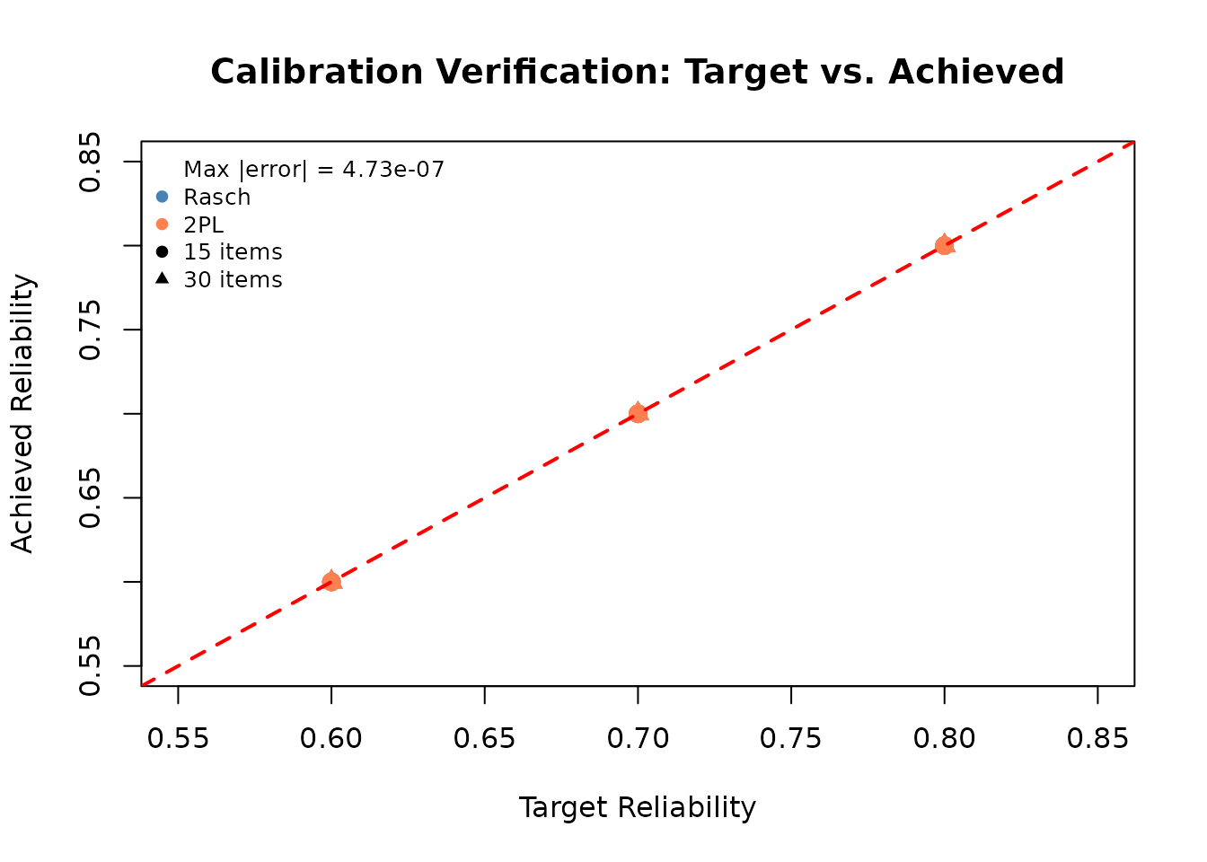

Scatter plot of achieved reliability against target reliability with a diagonal reference line.

Verification plot: achieved versus target reliability across all feasible cells. Points near the diagonal indicate precise calibration.

Points near the diagonal confirm a small numerical residual on the calibration quadrature. They do not replace an independent Monte Carlo holdout or an estimator-based response-data check.

External validation with TAM

For an estimator-based external diagnostic in Rasch/2PL cells, you can also use the TAM helper. WLE and EAP use different estimators and variance bases from IRTsimrel’s analytic target, so finite-sample differences are expected. The helper requires TAM to be installed:

if (requireNamespace("TAM", quietly = TRUE)) {
  for (i in seq_len(nrow(design_feasible))) {
    tam_rel <- compute_reliability_tam(
      resp  = sim_data_list[[i]]$response_matrix,
      model = design_feasible$model[i],
      verbose = FALSE
    )

    cat(sprintf("Cell %2d: target = %.3f, WLE = %.3f, EAP = %.3f\n",
                i, design_feasible$reliability[i],
                tam_rel$rel_wle, tam_rel$rel_eap))
  }
}

See vignette("validation") for guidance on interpreting WLE vs. EAP reliability from TAM.

compute_reliability_tam() intentionally accepts Rasch/2PL only. For a 3PL diagnostic, the validated workflow fits TAM::tam.mml.3pl() directly and uses EAP output; tam.wle() was unsupported for that fitted object in the tested TAM version. Do not coerce the object to manufacture a 3PL WLE result.

Practical Considerations

Seed management for reproducibility

A reproducible simulation study requires two levels of seed management:

Calibration seed: controls the quadrature sample and item parameters. Reusing a seed across cells deliberately creates common random-number coupling where generators share a draw sequence; using a deterministic cell-specific seed instead makes each realized design distinct. State which strategy you use.
Replication seeds: for each replication r = 1, \ldots, R, pass seed = r (or another deterministic mapping) to simulate_response_data(). This ensures that each replication is independently reproducible.

The recommended pattern encodes both cell index and replication index in the seed:

# Recommended seed pattern
CALIB_SEED <- 42

for (cell in seq_len(n_cells)) {
  res <- eqc_calibrate(..., seed = CALIB_SEED)

  for (r in seq_len(R)) {
    sim <- simulate_response_data(res, n_persons = N,
                                   seed = 1000 * cell + r)
    # ... analysis ...
  }
}

Important: IRTsimrel saves and restores the .Random.seed state inside eqc_calibrate() and simulate_response_data() when a seed is specified. This means that setting a seed inside these functions does not affect the global RNG state.

Result organization

Store simulation output in structured data frames. Pre-allocating the data frame is more efficient than growing it with rbind() inside the loop, but for clarity we show both patterns:

# Pre-allocate storage (efficient)
n_total <- nrow(design_feasible) * R
output <- data.frame(
  cell         = integer(n_total),
  rep          = integer(n_total),
  target_rho   = numeric(n_total),
  model        = character(n_total),
  n_items      = integer(n_total),
  latent_shape = character(n_total),
  rmse_beta    = numeric(n_total),
  bias_beta    = numeric(n_total),
  stringsAsFactors = FALSE
)

Computational scaling

Reliability-kernel work scales approximately with M \times I, but complete calibration time also depends on the number of topology evaluations and local roots. The analytic reducers automatically chunk large node-by-item products, bounding transient memory without changing the result. Response generation scales with N \times I. Because hardware and root topology matter, benchmark one representative cell on the machine used for production before projecting the full study runtime.

Parallelization

For large designs, cells can be calibrated in parallel because they are independent. The following pattern uses the future.apply package:

if (requireNamespace("future.apply", quietly = TRUE) &&
    requireNamespace("future", quietly = TRUE)) {
  future::plan(future::multisession, workers = 4)

  results_list <- future.apply::future_lapply(
    seq_len(nrow(design_feasible)),
    function(i) {
      d <- design_feasible[i, ]
      eqc_calibrate(
        target_rho   = d$reliability,
        n_items      = d$n_items,
        model        = d$model,
        latent_shape = d$latent_shape,
        item_source  = "parametric",
        reliability_metric = "info",
        M            = 10000L,
        seed         = 42
      )
    },
    future.seed = TRUE
  )
}

Replication loops can also be parallelized. Ensure that each parallel worker uses a unique seed:

# Parallelize replications within a cell
rep_results <- future.apply::future_lapply(seq_len(R), function(r) {
  sim <- simulate_response_data(
    result    = calib_result,
    n_persons = N,
    seed      = 1000 * cell_idx + r
  )
  # ... analysis ...
  # return(list(rmse = rmse, bias = bias))
}, future.seed = TRUE)

Reporting Standards

What to report in a simulation Methods section

A simulation study using IRTsimrel should report, at minimum:

Element	Example value
Package and version	IRTsimrel v0.3.0
Calibration algorithm	EQC
Reliability metric	Average-information (\tilde{\rho})
Target reliabilities	0.60, 0.70, 0.80
Test lengths	15, 30 items
IRT model	Rasch, 2PL (or 3PL with guessing specification)
Latent distribution	Normal, positively skewed
Item source	Parametric (Normal difficulties)
Quadrature size (M)	10,000
Replications per cell	500
Persons per replication	1,000
Seed management	Calibration seed = 42; replication seeds 1:500
Feasibility screening	All cells screened; N infeasible = 0
Root/scope contract	`lowest_increasing`; fixed form
Verification	Calibration residual plus independent holdout summary

Reporting checklist

State the target reliability levels and the metric used (info vs. msem).
Report the calibration algorithm and its key parameters (M, c_bounds, tol).
Document feasibility screening results.
Report the root policy, selected-root status, item scope, and maximum calibration residual across cells.
Describe the item parameter source and generation method.
State the latent distribution(s) and any shape parameters.
Report the number of replications and persons per replication.
Describe seed management for reproducibility.
For 3PL, report the lower-asymptote generator or fixed values and the D = 1 convention.
Distinguish calibration-quadrature, holdout, and estimator-based reliability results.
Cite Lee (2026) and the IRTsimrel package.

Results table template

The following table format is recommended for presenting results across a factorial design with reliability as a factor:

Model	I	Latent	\rho^*	c^*	RMSE(\beta)	Bias(\beta)	Coverage
Rasch	20	Normal	0.60	—	—	—	—
Rasch	20	Normal	0.70	—	—	—	—
Rasch	20	Normal	0.80	—	—	—	—
2PL	20	Normal	0.60	—	—	—	—
…	…	…	…	…	…	…	…

Methods paragraph template

Below is a complete, self-contained methods paragraph that can be adapted for your manuscript. Replace bracketed placeholders with your study’s values.

We employed a [3] (target reliability: [0.60, 0.70, 0.80]) \times [2] (test length: [15, 30] items) \times [2] (latent distribution: [normal, positively skewed]) \times [2] (model: [Rasch, 2PL]) fully crossed factorial design, yielding [24] conditions. Item response data were generated using the IRTsimrel R package (Lee, 2026). For each condition, the Empirical Quadrature Calibration (EQC) algorithm was used to select the lowest positive-slope crossing (root_policy = "lowest_increasing") at which the fixed-form empirical average-information reliability matched the target. Quadrature integration used M = 10{,}000 Monte Carlo abilities with one realized item form. All conditions were screened for feasibility prior to calibration; [0] conditions were infeasible and excluded. Item difficulties were drawn from N(0, 1); for the 2PL model, baseline discriminations were drawn from \text{LogNormal}(0, 0.3) with a Gaussian copula to induce the empirically observed negative difficulty-discrimination correlation (\rho_S = -0.3). For each of [500] replications per condition, N = [1{,}000] simulees were drawn from the specified latent distribution and binary responses were generated according to the IRT model. The maximum absolute residual on the calibration quadratures was [value], and independent holdout error was summarized as [value/interval]. All seeds were recorded for reproducibility.

Common Pitfalls and Solutions

Pitfall 1: Ignoring feasibility

Problem: you set target_rho = 0.99 with 5 items under the Rasch model, but EQC returns c_star at the upper bound with a warning.

Solution: always run check_feasibility() before calibration. If the target is infeasible, increase n_items, widen c_bounds, or reduce the target.

# Quick feasibility check before calibration
feas <- check_feasibility(
  n_items = 5, model = "rasch",
  target_rho = 0.99,
  c_bounds = c(0.1, 10), M = 5000L, seed = 42, verbose = FALSE
)
cat(sprintf("5-item Rasch: achievable rho_tilde range = [%.3f, %.3f]\n",
            feas$rho_range_info[1], feas$rho_range_info[2]))
#> 5-item Rasch: achievable rho_tilde range = [0.012, 0.948]
cat(sprintf("Target status: %s\n", feas$target_status_info))
#> Target status: above_upper

Pitfall 2: Metric confusion

Problem: you calibrate with reliability_metric = "info" and validate with the MSEM-based metric, finding a discrepancy.

Solution: by Jensen’s inequality, \tilde{\rho} \geq \bar{w} on the same population/grid basis. Always compare like with like. The recommended workflow uses "info" throughout. If you need to report both metrics, compute them using compute_rho_both():

# Compute both metrics from a single calibration
both <- compute_rho_both(
  c         = eqc_rasch$c_star,
  theta_vec = eqc_rasch$theta_quad,
  beta_vec  = eqc_rasch$beta_vec,
  lambda_base = eqc_rasch$lambda_base,
  theta_var = eqc_rasch$theta_var
)
cat(sprintf("rho_tilde (info): %.4f\n", both$rho_tilde))
#> rho_tilde (info): 0.8000
cat(sprintf("rho_bar   (msem): %.4f\n", both$rho_bar))
#> rho_bar   (msem): 0.7893
cat(sprintf("Gap (Jensen):     %.4f\n", both$rho_tilde - both$rho_bar))
#> Gap (Jensen):     0.0107

Pitfall 3: Insufficient quadrature size (M)

Problem: changing the seed or quadrature size changes the empirical root enough to affect conclusions.

Solution: increase M and evaluate the calibrated design on independent theta draws. A fixed seed makes a given configuration exactly reproducible, but does not remove Monte Carlo approximation error. Choose M through a problem-specific sensitivity check rather than a universal cutoff.

Pitfall 4: c_bounds too narrow

Problem: no admissible root is detected within the configured c_bounds. An infeasible EQC result reports the closest resolved point, which can be a boundary or an interior extremum; endpoint values alone do not define the attainable range.

Solution: inspect misc$rho_range, misc$topology, its root and extremum tables, and calibration_status. Expand c_bounds only when a wider discrimination scale is substantively defensible, then rerun the topology scan; do not infer feasibility merely from misc$rho_bounds.

Pitfall 5: Latent shape effects on reliability

Problem: calibrating under "normal" but generating data under "bimodal" gives achieved reliability different from the target.

Solution: the calibration and data generation must use the same latent distribution. If you intentionally mismatch them (e.g., to study robustness as in Case Study 2 of vignette("case-studies")), document and report an independently evaluated reliability estimate under the mismatched distribution.

Pitfall 6: Finite-sample deviation

Problem: with N = 100 persons, the sample reliability (e.g., from TAM) deviates substantially from the population target.

Solution: finite-sample deviation is expected and often shrinks at a root-N scale under regular conditions, but estimator bias, priors, and model fit also matter. Choose N through replication-based precision analysis and report the analytic target separately from empirical WLE/EAP diagnostics.

Publication-Ready Methods Text

Below is a second example methods paragraph, this time for a simpler two-factor design. Adapt the template by filling in your study’s values.

Item response data were generated using the IRTsimrel R package (v0.3.0; Lee, 2026). A 3 (target reliability: 0.60, 0.70, 0.80) x 2 (model: Rasch, 2PL) factorial design was employed with I = 20 items and a standard normal latent distribution. For each of the six conditions, the Empirical Quadrature Calibration (EQC) algorithm was used with M = 10{,}000 quadrature points and root_policy = "lowest_increasing" to select a discrimination scaling factor c^* matching the target fixed-form empirical average-information reliability \tilde{\rho}^*. Item difficulties were drawn from N(0, 1); for the 2PL model, baseline discriminations from \text{LogNormal}(0, 0.3). All conditions were verified feasible prior to calibration. For each of R = 500 replications per condition, N = 1{,}000 persons were drawn from N(0, 1) and binary responses generated according to the IRT model. The maximum calibration-quadrature residual was [value]; an independent holdout evaluation gave [summary].

Summary and Cross-References

This vignette presented a complete workflow for designing IRT simulation studies with reliability as a controlled design factor:

Build a factorial design with expand.grid().
Screen all cells for feasibility with check_feasibility().
Visualize reliability curves with rho_curve().
Batch-calibrate with eqc_calibrate().
Generate data with simulate_response_data().
Verify calibration accuracy.
Report following the guidelines above.

The key takeaway: reliability is not just an outcome to be measured after the fact; it is a design parameter to be specified, controlled, and reported from the outset. IRTsimrel makes this easy and precise.

For related topics, see:

vignette("introduction") – package overview and quick start.
vignette("algorithm-eqc") – deep dive into Algorithm 1 (EQC).
vignette("algorithm-sac") – Algorithm 2 (SAC) for independent validation.
vignette("item-parameters") – generating realistic item parameters.
vignette("latent-distributions") – working with non-normal latent distributions.
vignette("validation") – validation procedures and TAM integration.
vignette("case-studies") – publication-ready simulation templates.

References

Lee, J.-H. (2026). Reliability-Targeted Simulation of Item Response Data: Solving the Inverse Design Problem. arXiv:2512.16012v2. https://doi.org/10.48550/arXiv.2512.16012

Robbins, H., & Monro, S. (1951). A stochastic approximation method. The Annals of Mathematical Statistics, 22(3), 400–407.

JoonHo Lee (jlee296@ua.edu)

2026-08-22