14  Evidence quality

The claims of the preceding chapters lean on machinery: samplers that must have mixed, replication that must have been sufficient, labels whose error rates must be known, and locked sensitivity analyses that must be reported whether or not they flatter the primary specification. This chapter is that machinery’s account of itself. It reports convergence and inclusion, the DP arms’ cluster behavior, replication adequacy and the realized operating characteristic, interval-width mechanics, and the sensitivity grid, including the one place a registered conclusion visibly weakens.

14.1 Convergence and inclusion

All 7,200 fits completed and all entered the analysis under the locked inclusion policy; there were no exclusions and no reruns. Diagnostics are computed on the full reporting parameter set (person abilities, difficulties, and discriminations where present) as rank-normalized split R-hat with bulk and tail effective sample sizes. The median across fits of each fit’s worst R-hat is 1.00314; 186 fits (2.6%) crossed the 1.01 warning line, none crossed the 1.05 hard line, and 7,014 fits pass the stricter all-thresholds screen used by the strict-pass sensitivity below.

Table 14.1: Convergence and effective-sample-size roll-up by arm and family. Source: tables/T-convergence.rds.

Arm	Fits	Median max R-hat	R-hat > 1.01	Median bulk ESS	Strict pass
2PL
DP broad	1200	1.0033	56	6836	1144
DP focused	1200	1.0033	71	6798	1129
Gaussian	1200	1.0036	56	5592	1144
Rasch
DP broad	1200	1.0025	0	5106	1200
DP focused	1200	1.0025	0	5147	1200
Gaussian	1200	1.0037	3	3310	1197
Source: d_chain_convergence_rows.tsv via conv_rows.rds. Rank-normalized split R-hat over the full reporting parameter set; 0 hard failures and 0 exclusions among 7,200 fits under locked inclusion policy REQ-07d (hard threshold R-hat > 1.05; warnings are retained).

One number in the table deserves its sentence, because it reverses a defect of the previous study version: the arms’ effective sample sizes are now ordered DP above Gaussian (medians of roughly 5,100 to 6,800 against 3,300 to 5,600), reflecting the DP arms’ doubled retained draws. In V2 the DP arm had been the precision laggard, which contaminated arm comparisons with differential Monte Carlo error; the V3 budgets were set to prevent that, and did.

14.2 The DP prior’s clusters

Figure 14.1: Occupied-cluster counts increase substantially with sample size. Boxplots show the fit-level posterior median number of occupied clusters in the focused-DP arm; printed values are shape-specific medians. For bimodal, normal and skewed populations respectively, medians across N = 50, 100, 200 and 500 are 3/4/6/12, 3/4/7/16 and 3/4/6/13. Pooled over shape, the corresponding medians are 3, 4, 7, 14. The truncation guard registered pressure in 5 of 4,800 DP fits across both DP arms. Counts alone describe occupancy and do not identify component locations, weights, or which components represent the population modes.

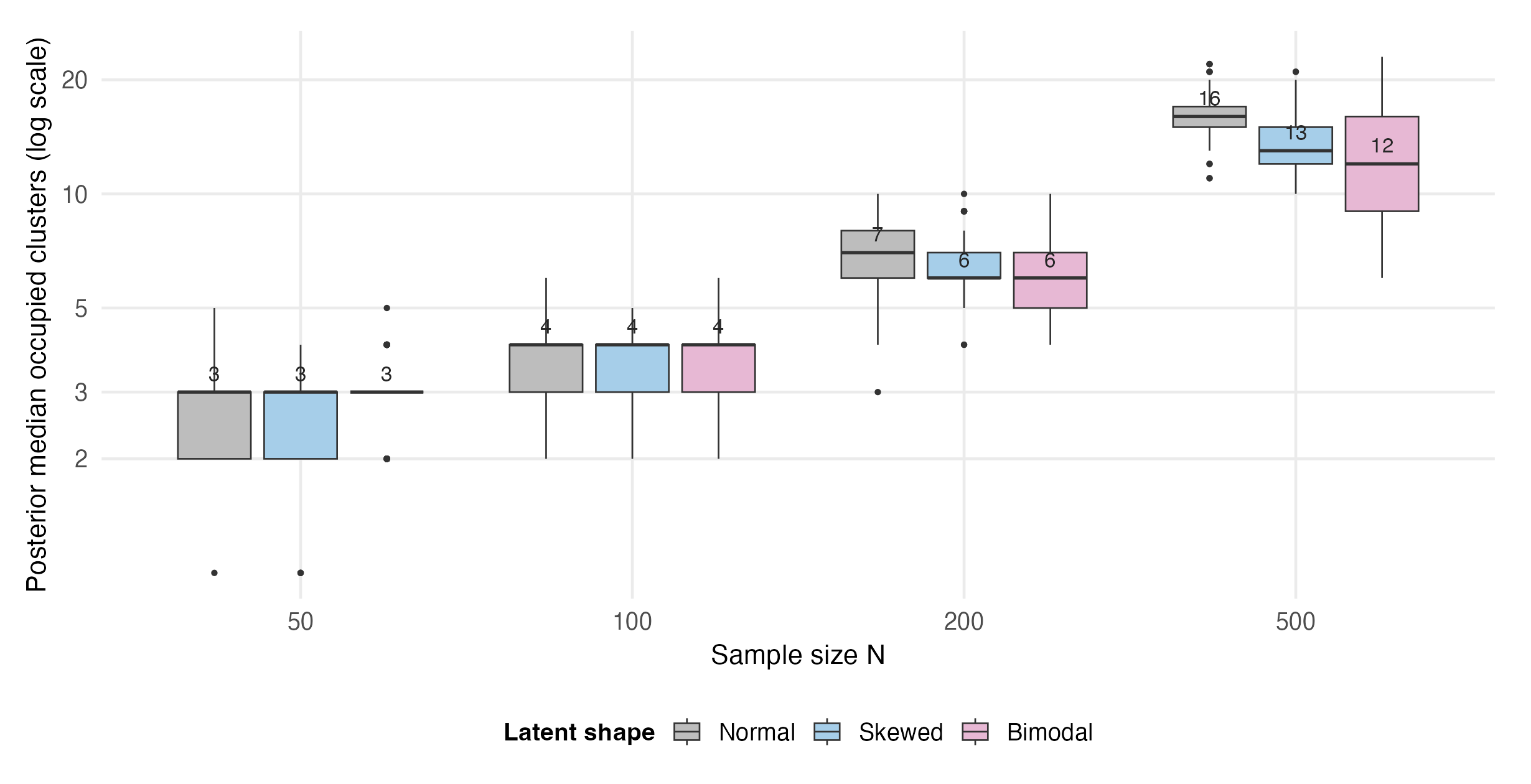
The focused arm’s posterior median occupied-cluster count increases with N. The medians for bimodal, normal and skewed populations are 3/3/3 at N = 50, 4/4/4 at N = 100, 6/7/6 at N = 200, and 12/16/13 at N = 500; pooled over shape they are 3, 4, 7 and 14. The truncation guard registered pressure in 5 of 4,800 DP fits. This diagnostic records occupancy only. It does not show component locations or weights and therefore cannot establish how many components represent a bimodal population.

14.3 Replication adequacy and the realized operating characteristic

The design’s replication promise was audited twice. Addendum 004 is the archival source for the pre-analysis trigger result: 12.5 percent of evaluable normal-control cells were ambiguous against its 20 percent threshold. The optional, direction-blind replication-extension route therefore did not activate; the locked wording ladder was a separate rule. After the wave, all six registered contrasts met their adequacy targets with claim_wording_step = full:

Table 14.2: Replication adequacy per contrast, evaluated against preregistered half-width targets. Source: tables/T-adequacy.rds.

Contrast	Cells	Median half-width	Target	Status	Wording step
contrast_cb_vs_pm	120	0.040	0.100	replication_adequate	full
contrast_dp_broad_gr_vs_dp_focused_gr	120	0.020	0.100	replication_adequate	full
contrast_dp_broad_gr_vs_gaussian_gr	120	0.068	0.100	replication_adequate	full
contrast_dp_focused_gr_vs_gaussian_gr	120	0.069	0.100	replication_adequate	full
contrast_dp_msel_safety	120	0.028	0.100	replication_adequate	full
contrast_normal_control_dp_vs_gaussian	40	0.078	0.100	replication_adequate	full
Results source: replication_adequacy_rows.tsv; all 6 contrast rows retain claim_wording_step = 'full'. Registry source: Addendum 004 was logged with 1,798 production fits complete but no production analyzer or outcome. It added an optional, direction-blind replication-extension route; the locked wording ladder already existed, and the trigger did not fire.

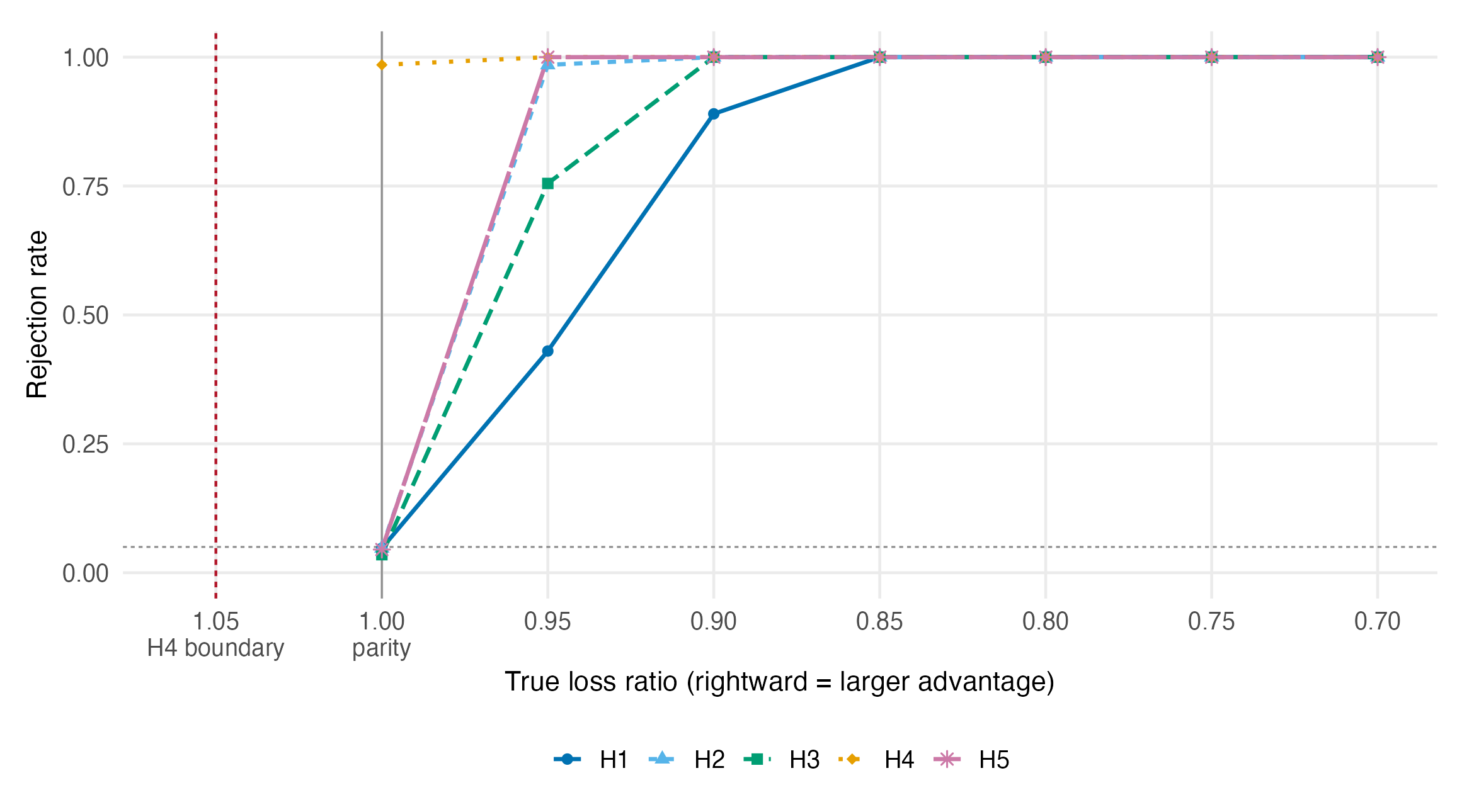
The realized operating characteristic (Figure 14.2) was computed after the wave from the achieved replicate variability, per the F-12 requirement, rather than from planning assumptions. At the parity null, H1, H2, H3 and H5 have rejection rates of 0.035 to 0.048 against the nominal 0.05; H4 instead has its non-inferiority null boundary at 1.05, shown separately in the figure. The normal-cell false-win rate is 0.008 against the 0.05 cap, and every hypothesis reaches full power by a true ratio of 0.85; the observed primary effects sit at 0.80 or better. The design was, in realized fact and not only in plan, able to detect what it claims to have detected and calibrated where it claims calibration.

Figure 14.2: The realized design rejects essentially always at the effects the study observed, and at the preregistered rates under the null. Realized operating characteristic computed after the wave from the achieved replicate variability (400 simulations per point, maximum Monte Carlo SE 0.025): rejection rates for each primary hypothesis against the true loss ratio. The grey line at ratio 1 is the parity null for H1, H2, H3 and H5; the separate red dashed line and labeled axis tick at 1.05 mark H4’s non-inferiority null boundary. At ratio 1 the rates are 0.035 to 0.048 against the nominal 0.05 (H4’s 0.985 at ratio 1 is correct behavior because ratio 1 is inside its non-inferiority alternative). Every hypothesis reaches full power by ratio 0.85; the observed primary effects sit at 0.80 or better.

14.4 Why the flag count falls without interval narrowing

Figure 14.3: The declining flag count is not caused by narrower intervals. Each point is one primary- contrast cell. Panel (a) plots its 95% hierarchical-bootstrap interval width on the log-ratio scale; the black median rises from 0.130 at N = 50 to 0.214 at N = 500. Raw-ratio median widths are 0.123, 0.137, 0.156 and 0.147, so that alternative scale does not show monotone narrowing either. Panel (b) shows that the median absolute log effect grows from 0.058 to 0.303 while the flag counts at N = 50, 100, 200 and 500 are 20, 14, 12 and 11. The N pattern therefore reflects point estimates moving farther from parity, together with the interval and evidence-label thresholds; it cannot be attributed to shrinking intervals alone.

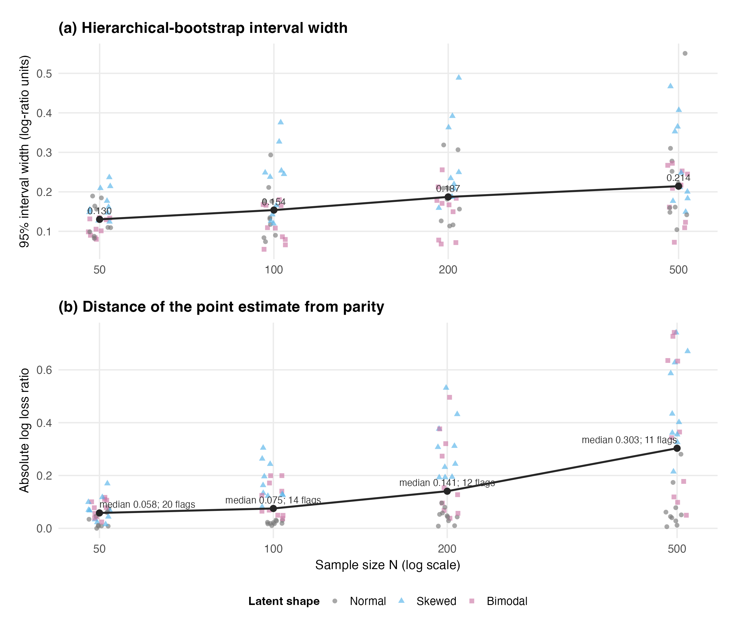
The evidence map’s flag counts are best read next to Figure 14.3. Median bootstrap width on the log-ratio scale increases across N: 0.130, 0.154, 0.187 and 0.214. On the raw-ratio scale the medians are 0.123, 0.137, 0.156 and 0.147, which is not monotone narrowing either. Meanwhile the median absolute log effect increases from 0.058 to 0.303 and the number of flags falls 20, 14, 12 and 11. The label gradient therefore cannot be explained by shrinking intervals; it reflects effects moving farther from parity together with the interval and point-threshold rules.

14.5 The sensitivity grid

The locked plan committed to three re-estimations of every registered hypothesis: equal condition weights, strict-pass fits only, and CR2 cluster-robust standard errors on the ten form families. Figure 14.4 overlays all four specifications; Chapter 15 holds the full table.

Figure 14.4: The registered conclusions survive every preregistered sensitivity, with one visible attenuation. Point estimates and 95% intervals for the five primary hypotheses (log loss-ratio responses) and the two secondary ones, under the locked primary specification and its three preregistered variants. This is an overview on one log axis: level log ratios (H1, H4 and H5), slopes (H2 and H6), and interaction or contrast coefficients (H3 and H7) have different units, so horizontal distances across those types are not direct effect-size comparisons. The red triangle marks H4’s non-inferiority margin at log 1.05; its intervals sit entirely below the margin in every variant. That average result coexists with seven bimodal reliability-0.5/0.6 cells with 5 to 14 percent higher MSEL; Chapter 12 reports their complete intervals and Addendum 006’s post-outcome timing. The one variant that moves a conclusion’s strength is strict-pass-only estimation of H5, which drops the focused-versus-broad advantage from -0.011 to -0.003 log units while remaining below zero (Holm-adjusted p = 0.040); the CR2 intervals are wide on 4 degrees of freedom by construction. Exact values appear in the preregistered-record chapter’s tables.

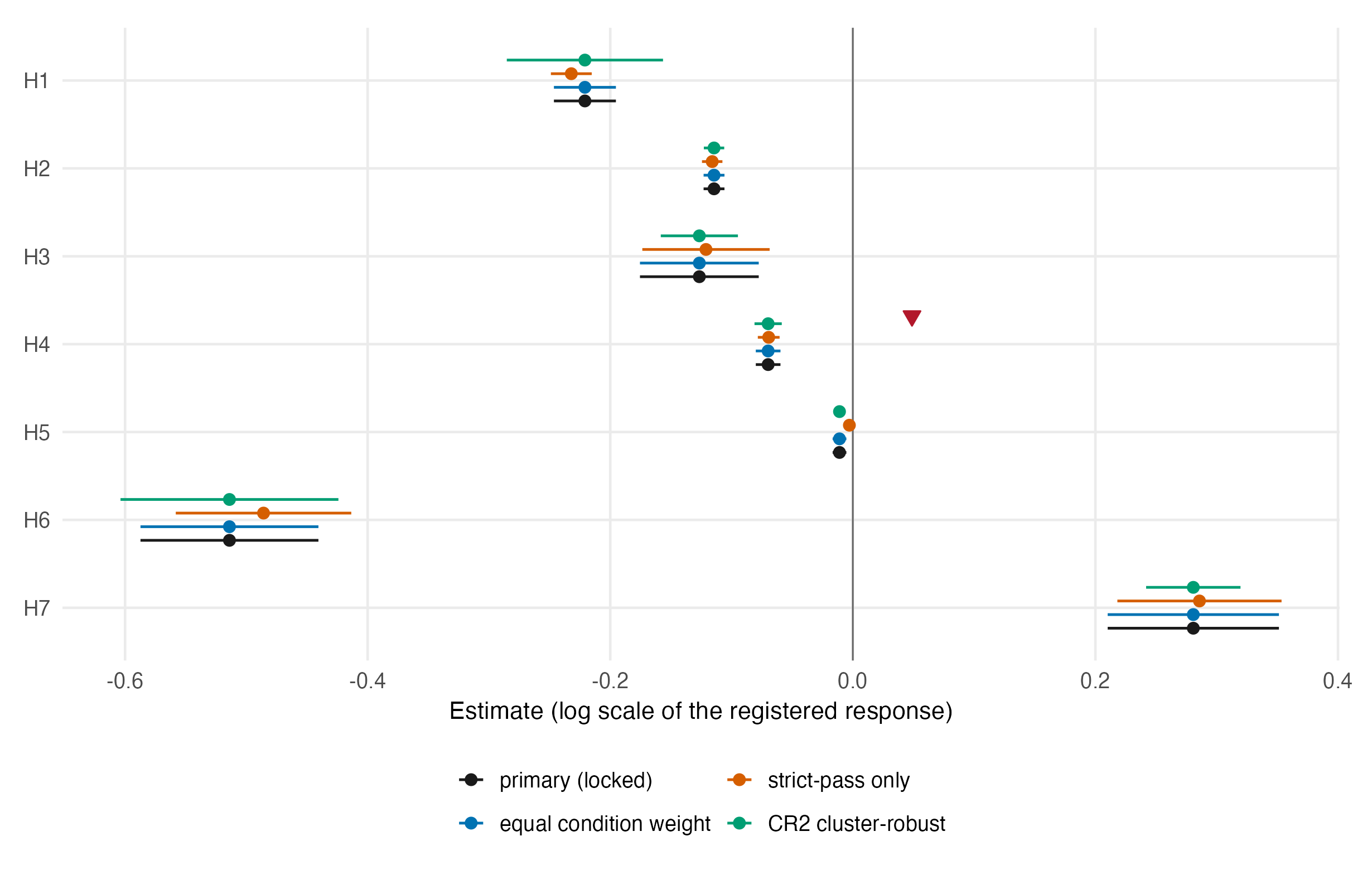
Equal condition weighting reproduces the primary estimates to several digits, as it must when cell sizes are balanced by design and nothing is excluded. The CR2 intervals widen on 4 degrees of freedom and issue no family verdict by convention; every interval nonetheless stays on its hypothesis’s side of zero, and H4’s average stays below its margin. That average does not erase the seven bimodal reliability-0.5/0.6 cells with 5 to 14 percent higher MSEL, ratios 1.052 to 1.138 with every interval excluding 1; Section 12.1 reports the complete cell-level table and Addendum 006’s post-outcome timing. The one substantive movement is H5 under strict-pass estimation: dropping the 186 warning fits attenuates the focused-versus-broad advantage from -0.011 to -0.003, a fifth its size, and the two-sided interval now includes zero ([-0.0061, 0.0004]) although the registered one-sided test still rejects (Holm-adjusted p \(= 0.040\)). A plausible reading is that part of the focused arm’s measured edge comes from fits where the broad arm mixed marginally worse rather than estimated worse; since H5 was already the family’s smallest effect, we label the focused arm’s superiority specification-dependent in magnitude and would not carry its point estimate into practice without that qualifier. H1 through H4, H6 and H7 move by at most a few percent of their values under every variant.

14.6 What this chapter establishes

The evidence base behaves: no exclusions, hard-clean convergence, arms whose precision no longer differs in the direction that once contaminated comparisons, adequacy targets met with the sealed trigger never fired, a realized operating characteristic that matches the plan’s promises, and a sensitivity grid whose only casualty is the magnitude, not the sign, of the family’s smallest effect. Readers who want the complete numerical record, including the exact p-values and every variant’s estimate, will find it collected in the next chapter.