10  Reliability and the observed recipe

The two previous chapters each ended at the same place: which combination of prior and summary is best depends on where the design sits along the reliability ladder. This chapter puts that dependence at the center. It reports the registered reliability-moderation hypothesis H6, decomposes its slope by shape (an exploratory step the registered contrast averages over), confronts the collinearity that the ladder builds into any such slope, and closes with the recipes: which studied combination performed best, per goal and reliability band, and the loss changes associated with other choices.

Only H6 is a registered contrast in this chapter. Its shape decomposition, companion model and the recipe table are exploratory syntheses of the simulated grid. They organize the observed patterns for practice but do not carry a preregistered error-rate guarantee or claim universality beyond the studied model families, shapes, information ladders and losses.

10.1 The registered gradient

H6, registered by Addendum 003 after P-3 and before any production fit, states that the flexible prior’s distribution-recovery advantage depends on achieved reliability within the non-normal domain. The fitted slope of the log loss ratio on centered achieved reliability, weighting the two non-normal shapes equally, is -0.514 (SE 0.037, 95% CI [-0.587, -0.441], Holm-adjusted p \(= 4.4 \times 10^{-41}\)). The sign convention needs one careful sentence: the response is log(DP loss / Gaussian loss), so a negative slope means the ratio falls, and the advantage therefore grows, as reliability rises. Its preregistered diagnostic, the same slope within the normal cells, is -0.029 with an interval covering zero ([-0.131, 0.074]), as a well-behaved control requires.

Addendum 005 fixes the interpretation of this result. H6 is moderation along the realized reliability ladder, on which achieved \(\bar\rho_J\), nested item count, global discrimination scale and finite-test information move together. The coefficient is confirmatory; a reliability-only, length-only or discrimination-only causal reading is not.

Figure 10.1: The reliability gradient is concentrated in the bimodal columns; the skewed columns show a flatter profile. Cell-level KS loss ratios replotted against each condition’s achieved information-based design coefficient, one line per sample size. In the bimodal columns the large-N lines dive as reliability rises (to 0.48 at reliability 0.8-0.9, N = 500 under Rasch); in the skewed columns the advantage is present but changes much less along the reliability axis, and under normality every line stays near parity (the preregistered diagnostic estimates that slope at -0.03 with an interval covering zero). The registered H6 slope of -0.51 (SE 0.04) averages the two non-normal shapes with equal weight, so it blends a steep bimodal gradient with a shallow skew one; the decomposition is reported in the text. The horizontal axis follows the realized nested-length plus cell-specific-discrimination ladder. Its components are highly collinear, so this display does not identify a causal effect of reliability, length, or discrimination separately.

10.2 The gradient decomposed

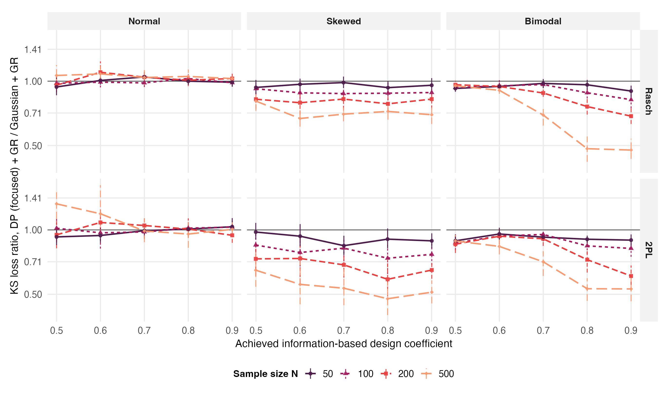
Figure 10.1 shows at once that the single H6 slope averages two quite different profiles. Refitting the registered model and reading the shape-specific slopes (an exploratory decomposition; the registered contrast is their equal-weight mean), we obtain -0.775 (SE 0.053) for the bimodal cells and -0.253 (SE 0.052) for the skewed cells, a threefold difference. (Our refit reproduces the registered pooled slope to -0.514 against -0.514, so the decomposition is read from the registered specification.) The observed asymmetry is clear; its mechanism is exploratory. One interpretation consistent with the sample-size fan of Section 8.3 is that broad asymmetry remains visible under coarser information, whereas separated modes require finer resolution. Because item count, \(c^\star\) and the shape of \(J(\theta)\) vary along the ladder, the decomposition does not identify which design component produces that difference. Descriptively, the H6 gradient is concentrated in the bimodal cells.

10.3 What the ladder cannot separate

Nested test length supplies the ladder’s largest structural change. Over the H6 estimation rows, the correlation between centered achieved reliability and centered log item count is 0.984. It is nevertheless incorrect to call the two variables identical: every model-by-form-by-tier-by-shape cell also has its own calibrated \(c^\star\), and matching the scalar \(\bar\rho_J\) does not match the full information curve.

An exploratory companion model that adds log item count alongside achieved reliability returns a reliability slope of -0.670 (SE 0.228) and an item-count slope of 0.021 (SE 0.030). The variance inflation factor is 31, and the model does not independently randomize or isolate \(c^\star\). Its coefficients therefore do not partition the H6 association into causal components. A separating design would have to cross length and discrimination scale independently, with prespecified information-curve diagnostics, rather than use one to refine targets set coarsely by the other (Chapter 17). What this design supports unchanged is the registered H6 statement: the DP-to-Gaussian loss ratio varies along the achieved joint ladder at the reported slope (Section 4.3).

10.4 Recipes

The practical output of the study is a small table. For each inferential goal and reliability band, Figure 9.4 (previous chapter) fixes the summary; the winner map and the safety screen then describe where the flexible prior improved the studied losses. These conditional defaults apply to the simulated dichotomous, unidimensional setting: three latent shapes, N = 50–500, ladder tiers 0.5–0.9, and one item-bank template per Rasch/2PL family. Because tier, nested length and cell-specific \(c^\star\) move jointly, the entries are not laws of a scalar reliability intervention. Stated as grid-specific rules:

1. For individual scores within the studied grid, the posterior mean has the lowest loss at each tier among the summaries studied; the prior is close to irrelevant (half the MSEL winner cells are near-ties between priors), and this study shows no individual-accuracy advantage that would justify adding the flexible prior for this goal alone.

2. For ranks, within-cell differences among the studied estimator choices remain small across all five tiers (Chapter 13); position on the joint information ladder is the dominant observed predictor.

3. For distribution reporting at ladder tiers up to 0.7, Gaussian + GR is a defensible default among the studied combinations. The summary swap captures most of the attainable gain, the flexible prior adds little that is resolvable (bimodal) or a modest amount (skew, growing with N), and at the bimodal low-tier corner seven opportunity-region cells show 5 to 14 percent higher individual MSEL, ratios 1.052 to 1.138 with every interval excluding 1 (Chapter 12). The clearest flexible-prior improvement in this band occurs at large N under skew, where the DP arm’s distributional gain is resolved (ratios near .65 at N = 500 under the 2PL) and the safety screen is quiet.

4. For distribution reporting at ladder tiers 0.8 to 0.9 under the studied non-normal shapes, the flexible prior with GR generally has the lowest observed loss. This is the region where the levers compound, where the prior can overtake the summary (Section 9.4), and where ratios reach .48; the calibrated (focused) elicitation is preferable in principle but the focused arm’s estimated loss is only about one percent below the broad arm in the primary H5 contrast (-0.01099). Under strict-pass-only filtering the estimate attenuates to -0.00284 (two-sided 95% CI [-0.00610, 0.00042]; registered one-sided Holm \(p = 0.0399\)), so focused should be treated as a defensible default rather than a practically consequential winner.

5. Under a defensibly normal population, or when the goal mixes individual scores with distributional reporting and no shape diagnosis is available, the Gaussian prior with the goal-matched summary is the defensible default across the studied grid; the flexible prior’s normal controls include three resolved higher-loss cells (at most 32 percent on KS at one 2PL corner) and show no resolved distributional advantage.

Chapter Chapter 16 restates these rules from the practitioner’s side, with the decision sequence, loss tradeoffs and computational demands. These recipes describe how the observed estimator ordering changes along this study’s information ladder; they are hypotheses for transport to other test designs, not estimator laws.