| Condition | MSEL ratio | 95% CI | Label |
|---|---|---|---|
| 2PL, N = 500, reliability 0.5, bimodal | 1.138 | [1.115, 1.162] | block |
| 2PL, N = 200, reliability 0.5, bimodal | 1.122 | [1.095, 1.149] | block |
| Rasch, N = 200, reliability 0.5, bimodal | 1.094 | [1.048, 1.136] | caution |
| 2PL, N = 200, reliability 0.6, bimodal | 1.092 | [1.070, 1.116] | caution |
| Rasch, N = 500, reliability 0.5, bimodal | 1.076 | [1.059, 1.093] | caution |
| 2PL, N = 500, reliability 0.6, bimodal | 1.072 | [1.059, 1.084] | caution |
| Rasch, N = 200, reliability 0.6, bimodal | 1.052 | [1.030, 1.077] | caution |
| The complete cell-level disclosure accompanies the direct H4 record here; later summaries preserve the seven-cell warning and cross-reference this table. | |||
12 Individual-accuracy tradeoffs
Everything reported so far concerns how well an estimate set represents a population. This chapter evaluates the corresponding changes in the quantity most users of test scores care about first: the accuracy of each person’s own estimate. The analysis has a preregistered instrument (the H4 safety test), a registered interpretation that constrains how its result may be stated (Addendum 006), and a set of descriptive companions. This chapter gives the complete confirmatory disclosure: all seven flagged cells, their intervals, and the addendum’s post-outcome timing. Elsewhere the book preserves the substantive warning in concise form and points here for the full record; post-registration analyses remain available as exploratory evidence rather than being forced into the confirmatory reporting template.
The findings in this chapter compare the study’s three priors and three summaries for dichotomous, unidimensional Rasch/2PL data over three latent shapes, N = 50–500 and joint length-plus-\(c^\star\) ladder tiers 0.5–0.9, using one item-bank template per family. They describe individual-accuracy changes within that grid, not penalties guaranteed for other item banks, response formats, dimensions or information regimes.
12.1 The safety result, stated as registered
H4 is a non-inferiority test on the opportunity region (non-normal shapes, N of 200 or 500): it asks whether the flexible pipeline’s mean squared-error loss ratio against Gaussian + GR stays below a margin of 1.05 in mean. It passes: the mean log ratio is -0.070 (95% CI [-0.080, -0.060]), with one-sided upper 95% bound -0.061 against the margin log(1.05) = 0.0488 (Holm-adjusted p \(= 2.3 \times 10^{-23}\)). On average over the opportunity region the flexible pipeline is not merely non-inferior for individuals but better, by about 7 percent.
The registered interpretation forbids leaving the statement there, because the average conceals a structured minority. The cell-level safety screen labels 33 of the 40 opportunity cells pass, 5 caution (ratio 1.05 to 1.10) and 2 block (above 1.10), and the seven flagged cells are not noise: every one is a bimodal population at reliability 0.5 or 0.6, and every one’s bootstrap interval excludes 1.
The largest ratio is 1.138 (2PL, N = 500, reliability 0.5). Addendum 006, which fixed this interpretation, was written after the production results were known and says so in its own text; its constraint is a wording constraint on H4 and leaves the distributional-recovery claims untouched, since they rest on different responses. We note also, as the addendum requires, that the harm’s location is itself a finding: the earlier V2 study led us to anticipate individual-accuracy harm under skew at N = 50, and the region that actually fired is bimodal at large N and low reliability, which is not the anticipated crossover but a different phenomenon.
12.2 Where individual accuracy changes
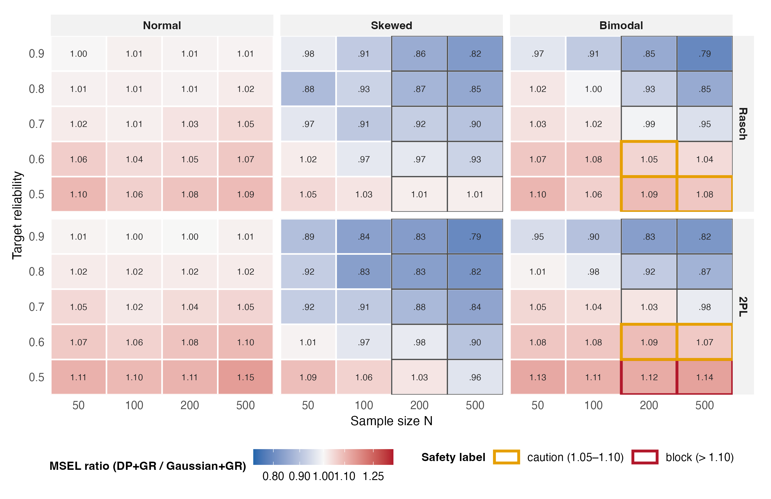
Figure 12.1 shows why the average and the flags coexist. Across the skewed columns and the high-reliability bimodal rows the tiles are blue: where the flexible prior can see the true shape, placing mass correctly helps each individual too, by up to 21 percent. The red region is confined to bimodal populations below reliability 0.7, strengthening with N. The mechanism is the geometry of shrinkage under a two-cluster prior. At low reliability each likelihood is wide, and a prior that has learned two modes pulls each posterior mean toward the nearer mode; when the person actually sits between the modes, squared error would prefer the conservative central shrinkage of the Gaussian prior. More data sharpens the prior’s conviction about the modes without sharpening any single person’s likelihood, which is why the MSEL increase grows with N in these cells. The same placement of mass can reduce KS loss, and Figure 12.2 displays the joint KS–MSEL changes: the flagged cells sit in the quadrant where KS loss decreases while individual MSEL increases.
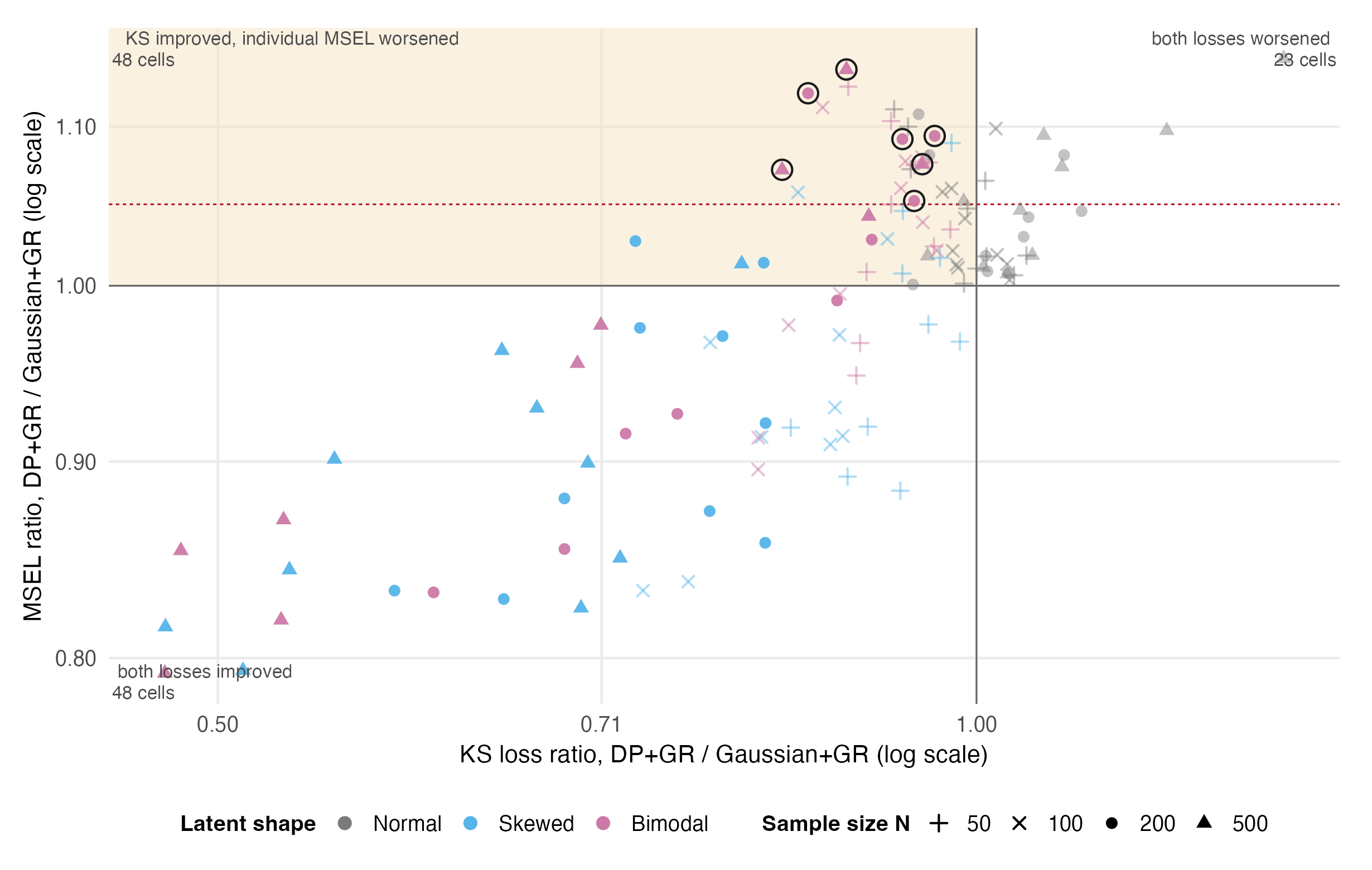
rr_point, the ratio of equal-form condition means for DP (focused) + GR against Gaussian + GR. The shaded upper-left quadrant contains 48 cells (40%) with lower KS loss and higher individual MSEL; the lower-left contains another 48 (40%) that improve both losses. Twenty-three cells (about 19%) worsen both, none improve individual loss while worsening distribution loss, and one normal Rasch cell lies on the KS ratio = 1 boundary. The dashed line is the 1.05 safety boundary. Circled points are the seven correctly flagged opportunity-region cells, all bimodal; solid symbols denote N = 200 or 500 and small crosses N = 50 or 100.
The quadrant census prevents the average safety result from erasing the trade-off: 48 of 120 cells improve both losses and exactly 48 gain on KS while worsening MSEL. Another 23 worsen both, none improve MSEL while worsening KS, and one normal Rasch cell lies exactly on the KS ratio = 1 boundary. The seven circled H4 flags remain the preregistered opportunity-region subset whose individual MSEL ratio crosses the safety thresholds.
12.3 The summaries’ individual-accuracy tradeoff
The posterior summary also changes individual accuracy. Holding the Gaussian prior fixed, the CB-versus-PM evidence map carries 99 flags of 120 cells, and Figure 12.3 tracks both alternatives against PM across the ladder. The median MSEL increase at reliability 0.5 is about 12 percent for CB and 20 percent for GR, and it declines with reliability, to inside the tie band for CB and to about 10 percent for GR at 0.9. This is the inverse image of the distributional penalties of Section 9.5: correcting ensemble spread and shape can increase individual squared error, with the magnitude related to how much shrinkage the summary reverses. The practical asymmetry is that GR’s distributional gains at low reliability are large (PM has a 73 percent geometric KS penalty relative to GR in the low band) while the median individual MSEL increase is smaller. Accordingly, within the simulated grid the recipes of Section 10.4 put GR first for distributional goals across the five tiers. A pipeline that feeds both goals from one estimate set must select the loss it prioritizes: all 240 displayed PM-versus-GR condition-mean point estimates occupy the dissociation quadrant, while H7 supplies the pooled registered test (Section 9.3).
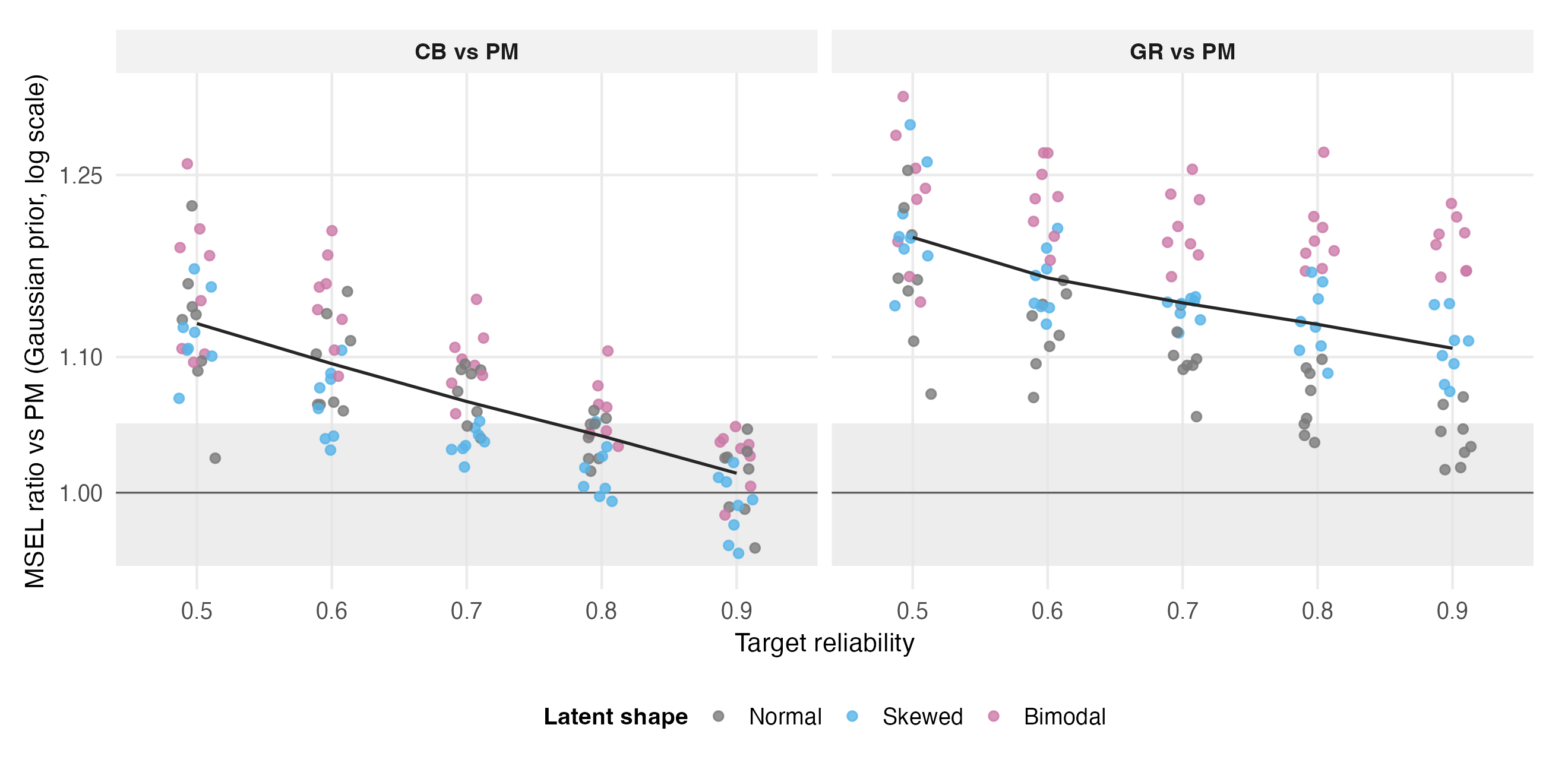
ratio_cells). The line traces the median across the 120 conditions by reliability tier, and the band marks 0.95 to 1.05. The locked CB-versus-PM evidence map uses the distinct rr_point ratio of equal-form condition means and labels 99 of 120 cells a flag; that count is not the plotted point estimand. Across the five simulated tiers, both alternatives have medians above 1; this is a statement about tier medians, not every cell. The median paired-geometric MSEL increase is about 12 percent for CB and 20 percent for GR at reliability 0.5; by reliability 0.9 the CB median falls inside the tie band while the GR median remains about 10 percent above PM, reflecting its different distributional objective rather than individual squared-error minimization.
12.4 What this chapter establishes
Averaged over its preregistered region, the flexible pipeline is better for individuals as well as for distributions. The coherent exception region comprises bimodal populations measured at reliability 0.6 and below; within it, individual MSEL is 5 to 14 percent higher, the increase grows with N, and all seven intervals exclude 1. Goal-matched summaries show their largest median individual MSEL increases at low information, with smaller increases higher on the calibrated joint ladder. These findings do not contradict the distributional results; the two sets of findings are two consequences of the same reallocation of shrinkage, and which side should govern a fitting choice depends on the goal, which is where the guidance of Chapter 16 begins.